Practical Exercise IV: Interpretable Machine Learning with mlr3 and DALEX
Veröffentlichungsdatum
22. Oktober 2024
For our empirical demonstration, we will use the DALEX/DALEXtra R packages (Biecek 2018), which come with a detailed online textbook (Biecek und Burzykowski 2021). An alternative is the iml package (Molnar u. a. 2018) with its excellent online companion book (Molnar 2019). The mlr3 e-book also contains a chapter on how to use both frameworks (Becker u. a. 2022). We use all IML methods on a RF model trained on the complete Sociability regression task. For a discussion on whether using IML on the complete dataset or using some combination of training and test sets, see chapter 8.5.2 in Molnar (2019).
Let’s repeat the earlier steps to load the dataset and create a random forest learner for the regression task.
First, we train the RF GraphLearner from earlier (which includes the imputation pipeline) on our complete Sociability task.
set.seed(123)rf_regr$train(task_Soci)
Then we construct an explainer object from the DALEXtra package, which takes as main inputs: model = a trained mlr3 model, data = the feature values of new observations for which predictions shall be computed (in our case these are the same data from our task appended with the gender variable), y = the target values for these new observations.1
library(DALEXtra)
Loading required package: DALEX
Welcome to DALEX (version: 2.4.3).
Find examples and detailed introduction at: http://ema.drwhy.ai/
Additional features will be available after installation of: ggpubr.
Use 'install_dependencies()' to get all suggested dependencies
Preparation of a new explainer is initiated
  -> model label       :  ranger explainer
  -> data              :  620  rows  1822  cols
  -> target variable   :  620  values
  -> predict function  :  yhat.GraphLearner  will be used (  default  )
  -> predicted values  :  No value for predict function target column. (  default  )
  -> model_info        :  package mlr3 , ver. 0.19.0 , task regression (  default  )
  -> predicted values  :  numerical, min =  -2.354667 , mean =  1.300549 , max =  4.364538
  -> residual function :  difference between y and yhat (  default  )
  -> residuals         :  numerical, min =  -2.437052 , mean =  -0.01940878 , max =  2.134029
  A new explainer has been created!
The explainer object can be used for all IML methods included in the DALEX/DALEXtra packages. To reduce the computational load for this tutorial, we only use a small subset of exemplary features for which we compute the IML methods. In practice, we would include all features from our task.
Permutation Variable Importance
To compute PVI, we use the model_parts function.
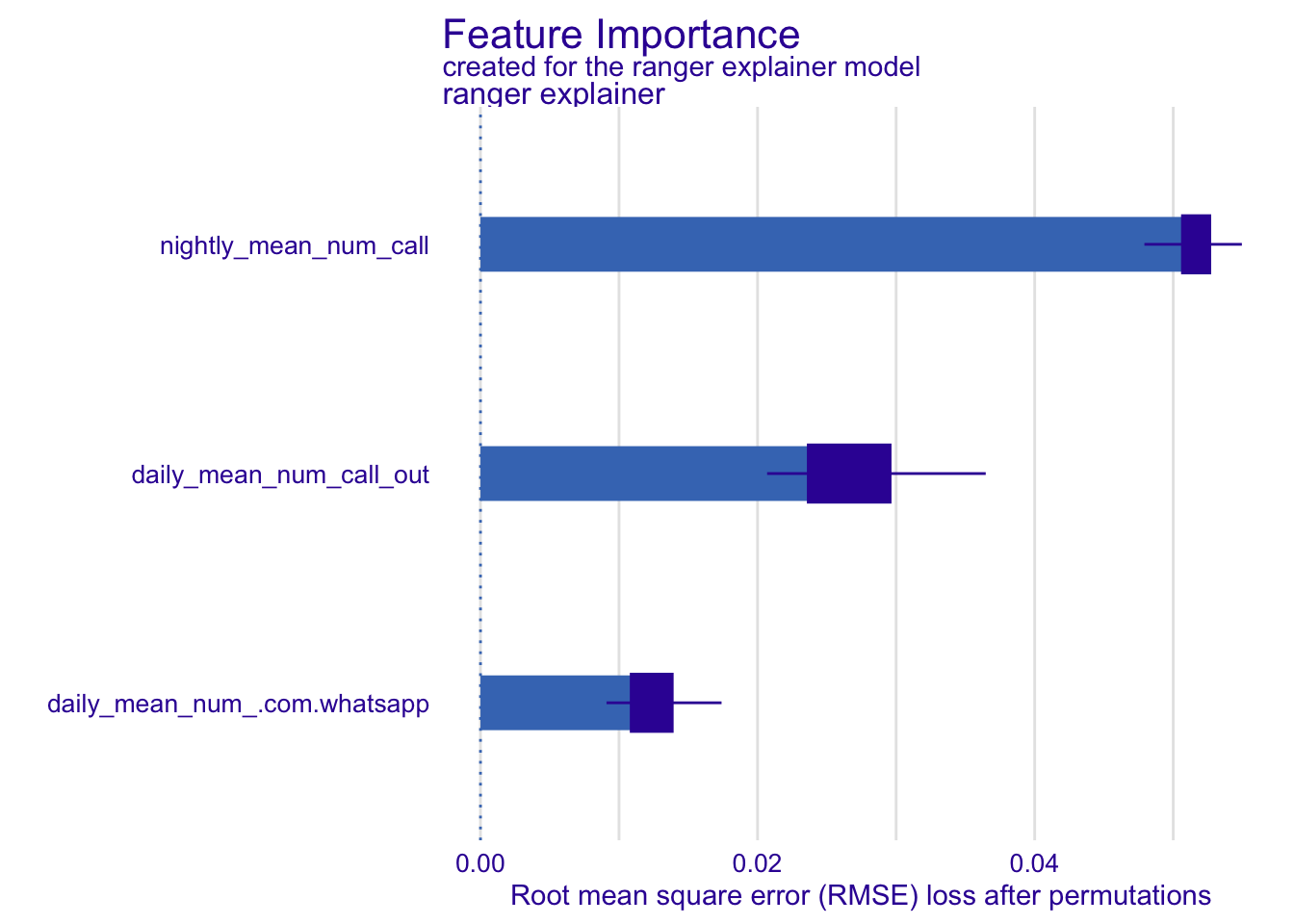
varimp <-model_parts(rf_exp, B =3, N =400, variables = exemplary_features, type ="difference")plot(varimp, show_boxplots =TRUE)
Permutation variable importance for three exemplary features based on the random forest model trained on the full Sociability regression task.
We only use a subset of observations (N) and a limited number of permutations (B) to reduce running times. In practice, we would increase the number of permutations and use all available observations. We plot the resulting objects (Figure @ref(fig:imp)), including boxplots that visualize the variability of feature importance across permutations. The default performance measure for regression tasks is the \(RMSE\). With type = "difference" in the model_parts function, the shuffled \(RMSE\) minus the unshuffled \(RMSE\) is displayed on the y-axis. This difference is more positive for more important features.
The PhoneStudy dataset consists of a very large number of features. In such settings, it can be more enlightening to interpret variable importance for groups of features (e.g., app categories, see Stachl u. a. 2020).2
Individual Conditional Expectation Profiles and Partial Dependence Plot
The model_profile function computes different measures to visually inspect feature effects. ICE is used when setting type = "partial" in model_profile and geom = "points" (or geom = "profiles") in the corresponding plot command.
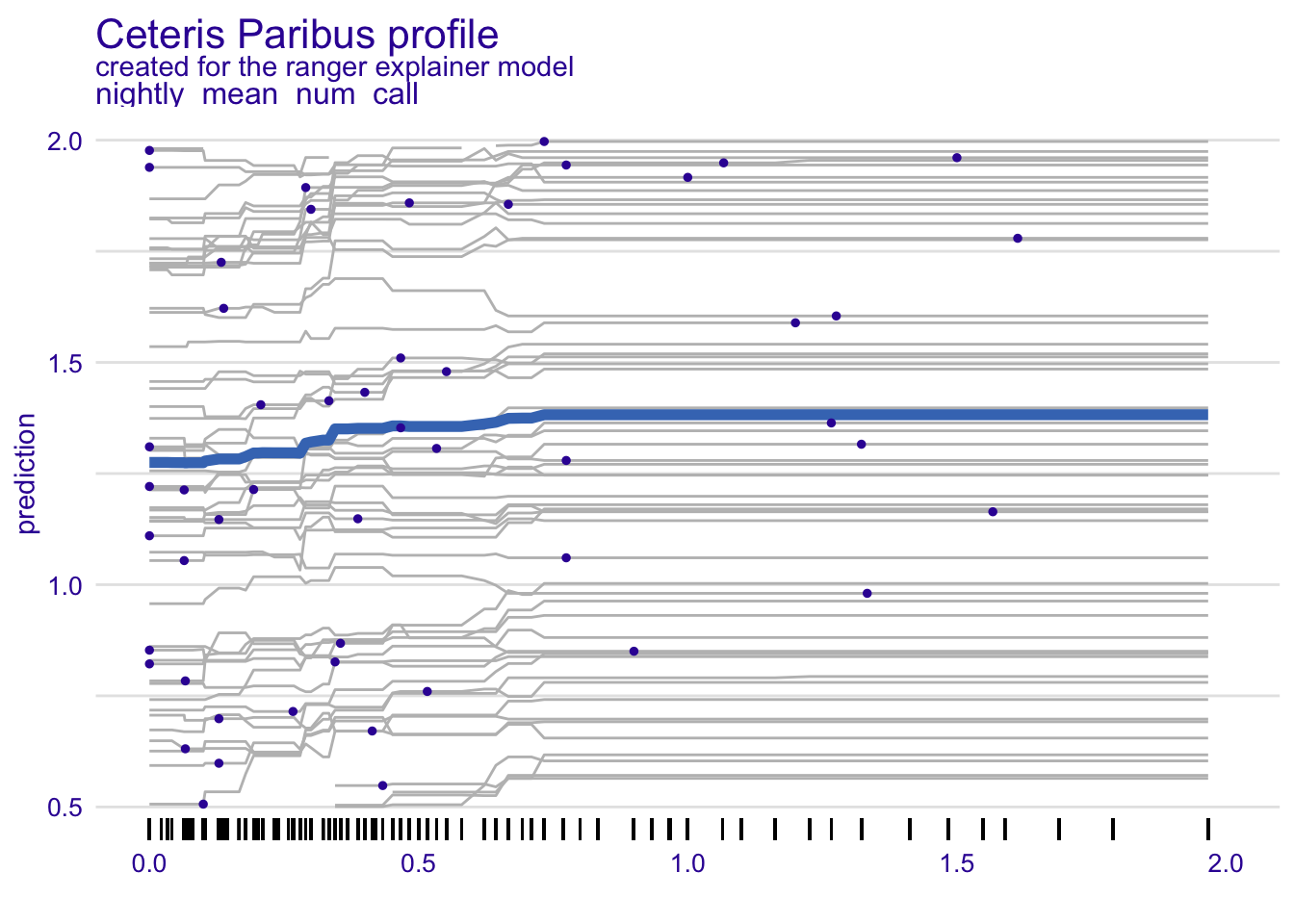
ice <-model_profile(rf_exp, variables = exemplary_features, N =100, center =FALSE, type ="partial")plot(ice, geom ="points", variables ="nightly_mean_num_call") +geom_rug(sides ="b") +xlim(0, 2) +ylim(0.5, 2)
Warning: Removed 4063 rows containing missing values or values outside the scale range
(`geom_line()`).
Warning: Removed 5 rows containing missing values or values outside the scale range
(`geom_line()`).
Warning: Removed 49 rows containing missing values or values outside the scale range
(`geom_point()`).
Individual conditional expectation profiles for the average number of telephone calls at night (nightly_mean_num_call) based on the random forest model trained on the full Sociability regression task.
Each ICE profile (i.e., each line in the plot) in Figure @ref(fig:ice) corresponds to one person in our dataset. It shows how the model’s predicted sociability for this person (on the y-axis) changes when we arbitrarily set the average number of telephone calls at night (nightly_mean_num_call; on the x-axis) to different values across the observed range, while keeping the person’s observed values on all other features. In this example, there is no sign for any strong interactions and the effect of all single features on the target seem quite weak (nightly_mean_num_call is already the most important feature measured by PVI, see Stachl u. a. 2020). The PD is already displayed in the ICE plot in Figure @ref(fig:ice) as the bold blue line. We could also request the PD by itself with type = "partial" in model_profile and geom = "aggregates" in the plot function. On average, we see a slight increase in predicted Sociability for a higher number of nightly calls. The corresponding ALE plot looks very similar and can be found in ESM 7.2.
Note that for these PhoneStudy examples, IML methods probably do not reveal causal effects: Personality theory would consider it unreasonable that some intervention that would simply call study participants at late hours, thereby increasing the average number of telephone calls at night (feature nightly_mean_num_call), would lead to an increase in those participants’ sociability.
Aspects of Model Fairness
To explore whether the predictive performance of our model differs between men and women, we compute predictive performance separately for each gender with the mlr3fairness companion package (Pfisterer u. a. 2022). When mlr3fairness is loaded before creating task_Soci, we can declare gender as a protected attribute (pta). We can then create groupwise performance measures that automatically take this variable into account.
The resampling results suggest that our model makes more accurate predictions for women (f) than for men (m). One plausible reason could be that the dataset contains more observations from women (61% women). The mlr3fairness package includes many more options for classification than for regression settings. Apart from evaluating fairness with different fairness metrics, it also contains methods to construct models with better fairness properties by using augmented ML models or debiasing methods.
To explore whether predicted sociability differentially depends on the value of the feature nightly_mean_num_call for men and women, the PD plot introduced earlier can be computed simultaneously for both genders, which we demonstrate in ESM 7.3. While the form of the relationship between the feature and the target predictions seems similar for both genders, the model generally predicts higher sociability for women than for men. Note that for both fairness analyses, the gender variable was not used as a feature when training the predictive model.
Literatur
Becker, Marc, Przemyslaw Biecek, Martin Binder, u. a. 2022. Flexible and Robust Machine Learning Using mlr3 in R. https://mlr3book.mlr-org.com/.
Biecek, Przemyslaw. 2018. „DALEX: Explainers for Complex Predictive Models in R“. Journal of Machine Learning Research 19 (84): 1–5. https://jmlr.org/papers/v19/18-416.html.
Biecek, Przemyslaw, und Tomasz Burzykowski. 2021. Explanatory Model Analysis. Chapman; Hall/CRC, New York. https://pbiecek.github.io/ema/.
Molnar, Christoph, Guiseppe Casalicchio, und Bernd Bischl. 2018. „iml: An R package for Interpretable Machine Learning“. Journal of Open Source Software 3: 786. https://doi.org/10.21105/joss.00786.
Pfisterer, Florian, Wei Siyi, und Michel Lang. 2022. mlr3fairness: Fairness Auditing and Debiasing for mlr3.
Stachl, Clemens, Quay Au, Ramona Schoedel, u. a. 2020. „Predicting personality from patterns of behavior collected with smartphones“. Proceedings of the National Academy of Sciences of the United States of America 117 (30): 17680–87. https://doi.org/10.1073/pnas.1920484117.
Fußnoten
Be careful when using explain_mlr3 with a classification task: y must to be a numeric variable with the positive class coded as 1 and the other coded with 0; predict_function_target_column must be set to the label of the positive class.↩︎