Practical Exercise III: Model Comparisons with Benchmark Experiments
Veröffentlichungsdatum
22. Oktober 2024
In our third exercise, we will conduct two benchmark experiments. The first benchmark experiment illustrates a classification task, the second a regression task. We will apply the RF from Module II, along with other learners. Besides a featureless learner, we also compare the RF to a so-called LASSO model (Tibshirani 1996) in our benchmark experiments. The LASSO is a linear regression (or classification) model that can effectively include a large number of features by shrinking the coefficients towards zero. This shrinkage also results in coefficients of exactly zero for unimportant features, thereby performing automatic variable selection because the corresponding features will not be taken into account when computing predictions. The results can be interpreted similar to ordinary linear or logistic regression because the LASSO can be seen as an alternative method to estimate the model parameters of these models. We have observed in our own ML applications that LASSO often performs comparably or even better than RF on survey data (e.g., Pargent und Albert-Von Der Gönna 2018). Thus, we recommend by default to include the LASSO into benchmark experiments when working with psychological data. A non-technical introduction to the LASSO is provided by James u. a. (2021).
Let’s repeat the earlier steps to load the dataset and prepare the binary classification task.
# load the packagelibrary(mlr3verse)
Loading required package: mlr3
# load the dataphonedata <-readRDS(file ="clusterdata.RDS")phonedata <- phonedata[complete.cases(phonedata$gender),]phonedata <- phonedata[, c(1:1821, 1823, 1837)]# create the regression tasktask_Soci <-as_task_regr(phonedata, id ="Sociability_Regr",target ="E2.Sociableness")task_Soci$set_col_roles("gender", remove_from ="feature")# create the classification taskphonedata$E2.Sociableness_bin <-ifelse( phonedata$E2.Sociableness >=median(phonedata$E2.Sociableness),"high", "low")phonedata$E2.Sociableness_bin <-as.factor(phonedata$E2.Sociableness_bin)task_Soci_bin <-as_task_classif(phonedata, id ="Sociability_Classif", target ="E2.Sociableness_bin", positive ="high")task_Soci_bin$set_col_roles("E2.Sociableness", remove_from ="feature")task_Soci_bin$set_col_roles("gender", remove_from ="feature")task_Soci_bin$set_col_roles("E2.Sociableness_bin", add_to ="stratum")
For our benchmark analysis, we reuse the task_Soci and task_Soci_bin objects we created earlier. We create GraphLearners fused with imputation (featureless learner, LASSO, and RF) for both a regression and a classification task. The featureless learner does not require imputation because it does not use any features.1
Because benchmark experiments easily become computationally intensive, we will use parallelization (speeding up computations, by using more than one core of the computer simultaneously) which is provided by the future package (Bengtsson 2021). To use parallelization with mlr3, the only steps are to load the future package, specify a parallelization plan (use strategy = "multisession" which should work on both Windows and Mac), and select the number of cores (you can type parallel::detectCores() to find out the maximum number of cores available on your computer). Parallelization will then be automatically used by mlr3 whenever possible. Note that even with a seed, parallel computations are sometimes not fully reproducible, which depends on technical peculiarities which are not specific to mlr3 or R.
Before we can actually compute the individual benchmark experiments for our regression and classification tasks, we have to declare our benchmark designs. These designs specify which learners shall be trained on which tasks and which resampling strategies should be used for each combination of learner \(\times\) task. We choose 10-fold CV to enable computation on smaller laptops in a reasonable time for our tutorial. In a real application, we would apply repeated CV here because performance estimates have a high variability for this example (notice how the estimates change when repeating the benchmark with different seeds). After running the experiments by calling the benchmark function for each task type, we turn off the parallelization by switching back to "sequential" mode.
INFO  [11:24:30.970] [mlr3] Running benchmark with 30 resampling iterations
INFO  [11:24:30.994] [mlr3] Applying learner 'classif.featureless' on task 'Sociability_Classif' (iter 1/10)
INFO  [11:24:31.016] [mlr3] Applying learner 'classif.featureless' on task 'Sociability_Classif' (iter 2/10)
INFO  [11:24:31.053] [mlr3] Applying learner 'classif.featureless' on task 'Sociability_Classif' (iter 3/10)
INFO  [11:24:31.087] [mlr3] Applying learner 'classif.featureless' on task 'Sociability_Classif' (iter 4/10)
INFO  [11:24:31.123] [mlr3] Applying learner 'classif.featureless' on task 'Sociability_Classif' (iter 5/10)
INFO  [11:24:31.163] [mlr3] Applying learner 'classif.featureless' on task 'Sociability_Classif' (iter 6/10)
INFO  [11:24:31.197] [mlr3] Applying learner 'classif.featureless' on task 'Sociability_Classif' (iter 7/10)
INFO  [11:24:31.232] [mlr3] Applying learner 'classif.featureless' on task 'Sociability_Classif' (iter 8/10)
INFO  [11:24:31.272] [mlr3] Applying learner 'classif.featureless' on task 'Sociability_Classif' (iter 9/10)
INFO  [11:24:31.306] [mlr3] Applying learner 'classif.featureless' on task 'Sociability_Classif' (iter 10/10)
INFO  [11:24:31.341] [mlr3] Applying learner 'imputemedian.classif.cv_glmnet' on task 'Sociability_Classif' (iter 1/10)
INFO  [11:24:31.377] [mlr3] Applying learner 'imputemedian.classif.cv_glmnet' on task 'Sociability_Classif' (iter 2/10)
INFO  [11:24:36.240] [mlr3] Applying learner 'imputemedian.classif.cv_glmnet' on task 'Sociability_Classif' (iter 3/10)
INFO  [11:24:36.720] [mlr3] Applying learner 'imputemedian.classif.cv_glmnet' on task 'Sociability_Classif' (iter 4/10)
INFO  [11:24:41.339] [mlr3] Applying learner 'imputemedian.classif.cv_glmnet' on task 'Sociability_Classif' (iter 5/10)
INFO  [11:24:42.133] [mlr3] Applying learner 'imputemedian.classif.cv_glmnet' on task 'Sociability_Classif' (iter 6/10)
INFO  [11:24:46.090] [mlr3] Applying learner 'imputemedian.classif.cv_glmnet' on task 'Sociability_Classif' (iter 7/10)
INFO  [11:24:47.122] [mlr3] Applying learner 'imputemedian.classif.cv_glmnet' on task 'Sociability_Classif' (iter 8/10)
INFO  [11:24:50.894] [mlr3] Applying learner 'imputemedian.classif.cv_glmnet' on task 'Sociability_Classif' (iter 9/10)
INFO  [11:24:52.749] [mlr3] Applying learner 'imputemedian.classif.cv_glmnet' on task 'Sociability_Classif' (iter 10/10)
INFO  [11:24:55.806] [mlr3] Applying learner 'imputemedian.classif.ranger' on task 'Sociability_Classif' (iter 1/10)
INFO  [11:24:57.712] [mlr3] Applying learner 'imputemedian.classif.ranger' on task 'Sociability_Classif' (iter 2/10)
INFO  [11:25:00.158] [mlr3] Applying learner 'imputemedian.classif.ranger' on task 'Sociability_Classif' (iter 3/10)
INFO  [11:25:02.893] [mlr3] Applying learner 'imputemedian.classif.ranger' on task 'Sociability_Classif' (iter 4/10)
INFO  [11:25:04.737] [mlr3] Applying learner 'imputemedian.classif.ranger' on task 'Sociability_Classif' (iter 5/10)
INFO  [11:25:08.294] [mlr3] Applying learner 'imputemedian.classif.ranger' on task 'Sociability_Classif' (iter 6/10)
INFO  [11:25:09.128] [mlr3] Applying learner 'imputemedian.classif.ranger' on task 'Sociability_Classif' (iter 7/10)
INFO  [11:25:13.478] [mlr3] Applying learner 'imputemedian.classif.ranger' on task 'Sociability_Classif' (iter 8/10)
INFO  [11:25:13.549] [mlr3] Applying learner 'imputemedian.classif.ranger' on task 'Sociability_Classif' (iter 9/10)
INFO  [11:25:17.992] [mlr3] Applying learner 'imputemedian.classif.ranger' on task 'Sociability_Classif' (iter 10/10)
INFO  [11:25:22.255] [mlr3] Finished benchmark
plan("sequential")
We choose an extended set of performance measures for our regression and classification benchmarks. For regression, we look at \(R^2\) and \(RMSE\) but also consider the Spearman correlation, which evaluates predictive performance by correlating the predictions with the true target values. Evaluating predictive performance with correlation measures is useful in practical applications in which we only care about ranking individuals based on the target (e.g., is this person rather more or less sociable compared to this other person) but the actual target values do not matter. Such settings frequently arise in psychological assessment (e.g., personnel selection, Stachl u. a. 2020). For classification, we not only look at \(MMCE\) but also consider \(SENS\) (i.e., true positive rate) and \(SPEC\) (i.e., true negative rate).
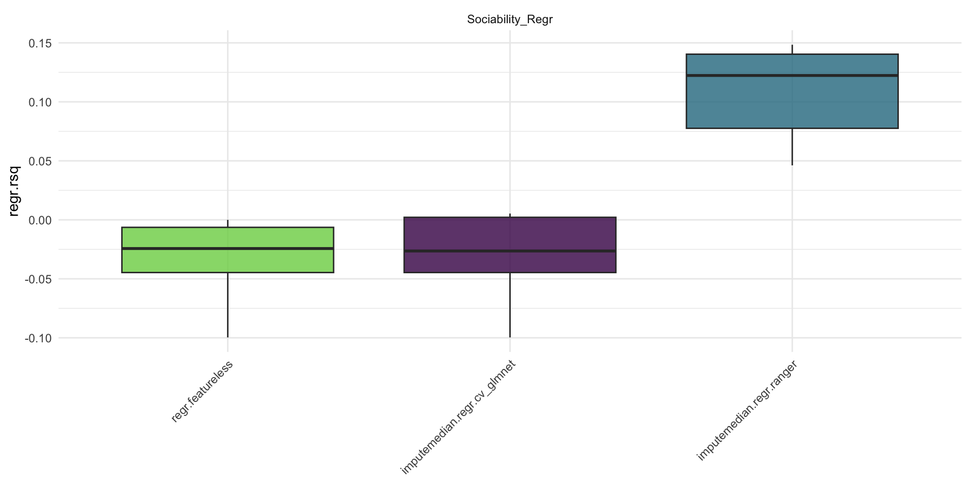
First, we compute aggregated performance for the regression benchmark with aggregate and print the results. We can also request a grouped boxplot for a specific performance measure, which is very useful because it also visualizes the variability of performance estimates across test sets.
bmr_regr <- bm_regr$aggregate(mes_regr)
Warning in cor(truth, response, method = "spearman"): the standard deviation is
zero
Warning in cor(truth, response, method = "spearman"): the standard deviation is
zero
Warning in cor(truth, response, method = "spearman"): the standard deviation is
zero
Warning in cor(truth, response, method = "spearman"): the standard deviation is
zero
Warning in cor(truth, response, method = "spearman"): the standard deviation is
zero
Warning in cor(truth, response, method = "spearman"): the standard deviation is
zero
Warning in cor(truth, response, method = "spearman"): the standard deviation is
zero
Warning in cor(truth, response, method = "spearman"): the standard deviation is
zero
Warning in cor(truth, response, method = "spearman"): the standard deviation is
zero
Warning in cor(truth, response, method = "spearman"): the standard deviation is
zero
Warning in cor(truth, response, method = "spearman"): the standard deviation is
zero
Warning in cor(truth, response, method = "spearman"): the standard deviation is
zero
Warning in cor(truth, response, method = "spearman"): the standard deviation is
zero
Warning in cor(truth, response, method = "spearman"): the standard deviation is
zero
Warning in cor(truth, response, method = "spearman"): the standard deviation is
zero
Boxplots displaying the results of the benchmark experiment of the Sociability regression task based on the PhoneStudy dataset. \(R^2\) was estimated with 10-fold cross-validation. Left: featureless learner, middle: LASSO, right: random forest.
It seems that the RF produces more accurate predictions than the LASSO and the featureless learner for all performance measures. Note that the Spearman correlation could not be computed for the LASSO and the featureless learner because both produced constant predictions for all observations within at least one fold. While this must always be the case for the featureless learner (i.e., constant prediction based on the target mean in the training set), it seems that the LASSO automatically removed all features from the model (i.e., constant prediction based on the model intercept). This observation reflects the bad performance of the LASSO, which cannot effectively use the information contained in the features in this example.
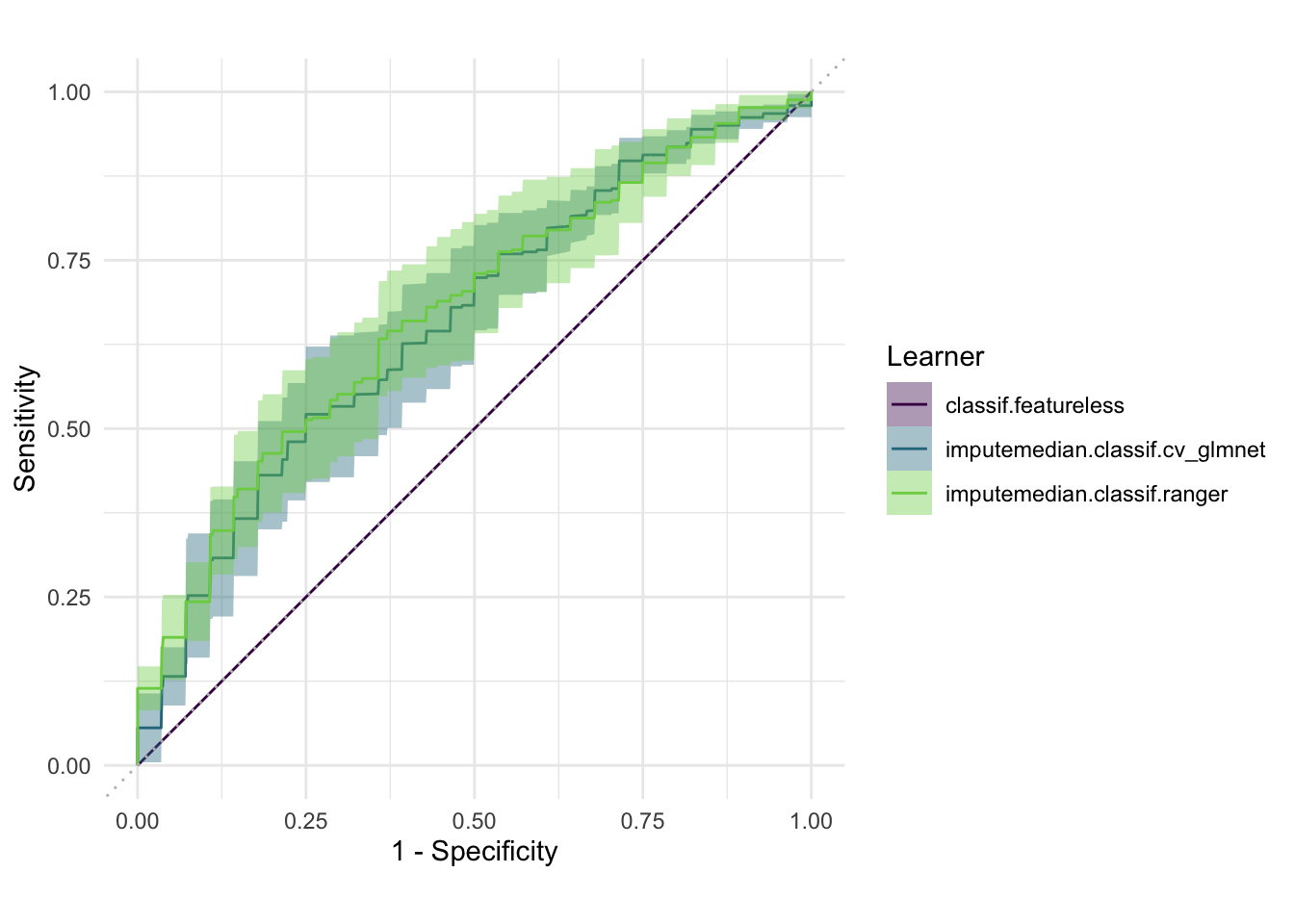
The commands to display benchmark results are similar for the classification benchmark. Instead of the grouped boxplot, we here show how to produce a simple ROC plot by calling autoplot(bm_classif, type = "roc").
ROC plot displaying the results of the benchmark analysis of the Sociability classification task based on the PhoneStudy dataset. ROC curves were estimated with 10-fold cross-validation. The shaded grey region visualizes the variability across test sets.
When looking at the results, we notice that while \(MMCE\) is very similar for RF and LASSO, the models slightly differ in their respective tradeoff of \(SENS\) and \(SPEC\). This finding exemplifies the need to consider other performance measures beyond mean classification error or accuracy in many applied classification settings, in which the practical cost of false positive and false negative predictions are not the same (Sterner u. a. 2021).
To practice with another benchmark example, ESM 6 contains mlr3 code to perform a benchmark experiment with the Titanic dataset.
BONUS EXERCISE:
If you want, you can follow up here with Practical Exercise IV on Interpretable Machine Learning with mlr3 and DALEX.
References
Becker, Marc, Przemyslaw Biecek, Martin Binder, u. a. 2022. Flexible and Robust Machine Learning Using mlr3 in R. https://mlr3book.mlr-org.com/.
Bengtsson, Henrik. 2021. „A Unifying Framework for Parallel and Distributed Processing in R using Futures“. The R Journal, Online-Vorab-Publikation. https://doi.org/10.32614/RJ-2021-048.
James, Gareth, Daniela Witten, Trevor Hastie, und Robert Tibshirani. 2021. An Introduction to StatisticalLearning: with Applications in R. New York: Springer.
Pargent, Florian, und Johannes Albert-Von Der Gönna. 2018. „Predictive Modeling with Psychological Panel Data“. Zeitschrift fur Psychologie / Journal of Psychology 226 (4): 246–58. https://doi.org/10.1027/2151-2604/a000343.
Stachl, Clemens, Florian Pargent, Sven Hilbert, u. a. 2020. „Personality Research and Assessment in the Era of Machine Learning“. European Journal of Personality 34 (5): 613–31. https://doi.org/10.1002/per.2257.
Sterner, Philipp, David Goretzko, und Florian Pargent. 2021. Everything has its Price: Foundations of Cost-Sensitive Learning and its Application in Psychology. PsyArXiv. https://doi.org/10.31234/osf.io/7asgz.
Tibshirani, Robert. 1996. „Regression Shrinkage and Selection via the Lasso“. Journal of the Royal Statistical Society. Series B (Methodological) 58 (1): 267–88. http://www.jstor.org/stable/2346178.
Fußnoten
We set the predict_type of the classification learners to "prob", which is only necessary because we want to show a ROC curve later. For more details on predict_type, we refer to the mlr3 e-book (Becker u. a. 2022).↩︎