1 + 8R Tutorial (Part 1): The Basics
How Does This Tutorial Work?
This tutorial is intended for students who have never worked with R and RStudio before, or who wish to refresh their memory by starting with the absolute basics again. The tutorial will guide you through the fundamentals of the statistics program R step by step. Using a statistical software such as R is required in various contexts related to studying and research. Thus, R is an important tool for empirical work, which will not only help you to understand statistical concepts better, but will also allow you to carry out statistical analyses yourself.
In this tutorial we will explain to you the structure and fundamental functioning of R and RStudio. You will find boxes of different colors throughout the tutorial:
NoteNote
In the blue boxes you will find useful hints, which explain the work with R and RStudio in more detail.
TipTip
In the green boxes we deal with further topics on the functionality of R and RStudio. If you want, you can skip these boxes at the first run, so that it is easier for you to focus on the basics.
WarningWarning
In the yellow boxes we point you to pitfalls and possible sources of error. Try to memorize these points especially so that R always does what you want.
CautionTry it out yourself!
In the orange boxes you will find a number of exercises. Please do all the exercises yourself on your own computer.
How to Use This Tutorial
Learning R is just like learning a new language. You have to repeat the content again and again until the learned can be applied in practice independently. Don’t be too strict on yourself and don’t expect to have already internalized all the content after working through the tutorial for the first time. Our tutorial is intended to encourage you to try out the presented content immediately. Therefore, we have repeatedly supplemented the text and our examples with images and small GIFs (short videos without sound) that explain how to use the program. The exercises presented in the red boxes are also a central part of the tutorial. In the first of these boxes, we will prompt you to install R and RStudio on your own computer. Our experience shows that mastering R and RStudio is only successful if you work with it yourself from the very beginning and revise the contents regularly.
Please do it! It will definitely be worth it!
1 First steps in R and R-Studio
R, as we use it, consists of two programs: R and RStudio. R and RStudio are not the same, but build on each other.
What is R?
![]()
- programming language with a focus on statistics, open-source and free
- The “engine”, the program that performs all our calculations
- Can do anything we need (and much more)
- Should be updated regularly
What is RStudio?
![]()
- Additional program (editor) for easier use of R, open-source and free
- Accesses R in the background, therefore it does not work without having R installed
- Can do anything R can, but is more user-friendly
- Should be updated regularly
1.1 Installation
NoteNote
If you are using a private computer it is helpful and necessary to know how to install programs on it. The individual steps depend on your respective computer and operating system. Since there are a lot of different computer and operating system models, we can’t offer a detailed guide for each variant for the program installation.
Please familiarize yourself with your device so that you can also install and use programs (“apps”) such as R and RStudio.
The following steps give a small overview of the most common ways to install the program:
Installation on Computers with Windows Operating System
Installation files are usually downloaded from Windows as an executable file with the .exe file extension. Double-clicking on this file will start the installer and you only have to follow the instructions on the screen.Installation on Computers with Mac Operating System
On a Mac, there are two variants for downloaded installation files, where the following steps differ. You can recognize these variants by the respective file extension, which is either “.pkg” (e.g. the program R) or “.dmg” (e.g. the program RStudio).
File Extension pkg
- Double-click on the downloaded installation file in the “Downloads” folder (it is displayed as an open postal package).
- Follow the instructions displayed on the screen.
File Extension dmg
- Downloading the DMG file: Most programs are downloaded from the manufacturer’s website as .dmg file. This file is usually found in the “Downloads” folder or on the desktop.
- Open the DMG file: Double-click the downloaded DMG file to mount it. A new window with the program icon appears. If no window appears, check your desktop - a “virtual drive” is displayed there.
- Drag-and-drop: Drag the program icon into the “Program Files” folder in the Finder. This step copies the application firmly to your system.
- Remove the virtual drive: Right-click the virtual drive on the desktop after copying and select “Eject” or press CMD+E to safely remove the drive.
- Security queries: When you open an application that has been downloaded from the Internet, macOS may display a security warning. Confirm that you trust the application by clicking “Open”.
Installation on Computers with Linux Operating System
If you’re using Linux as an operating system, you probably don’t need a guide of this kind… ;-)To install R, click [here] (https://posit.co/download/rstudio-desktop/) and then click 1: Install R. Then we have to select the correct version for our operating system, download and install it (like any other program).
To install RStudio afterwards, click [here] (https://posit.co/download/rstudio-desktop/) and then click 2: Install RStudio. This should automatically download the correct version for our operating system, which we can then install (like any other program).
CautionTry it out yourself!
Install R and RStudio on Your Computer.
Note: Unfortunately, an installation on tablets with iOS or Android operating system is not possible. Therefore, you need a laptop or desktop computer. Whether you’re a Mac, Windows or Linux user, doesn’t matter.
TipUpdating R and RStudio
R and RStudio should be updated regularly to ensure that we use the latest features and security updates. RStudio usually automatically reminds us when an update is available. You can use this reminder from RStudio to also install the latest version of R. Unfortunately, there is no automatic reminder from R itself.
Neither R nor RStudio can be updated automatically. To update R and RStudio, we simply go back to [the website from above] (https://posit.co/download/rstudio-desktop/) and download the latest version, as if we were installing the program for the first time.
R can be easily installed on Mac via the existing version. On Windows we need to manually uninstall the old version (e.g. via Start > Settings > Apps > Apps & Features), if we want to prevent multiple versions of R from being installed at the same time. Normally, RStudio will automatically find the latest version of R installed on your computer if you close RStudio completely and reopen it again.
RStudio can normally be installed on both Mac and Windows via the existing version without having to manually delete the old version.
After installing R and RStudio, we only work with RStudio. R itself does not have to be opened at any time (if you want, you can delete the desktop shortcut to R directly to avoid confusion with RStudio).
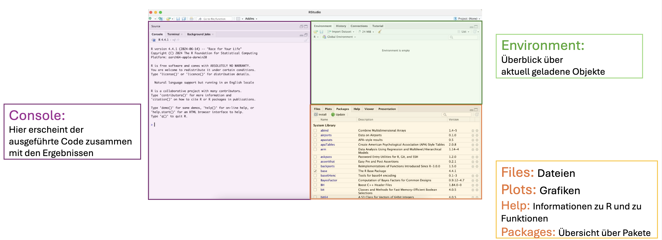
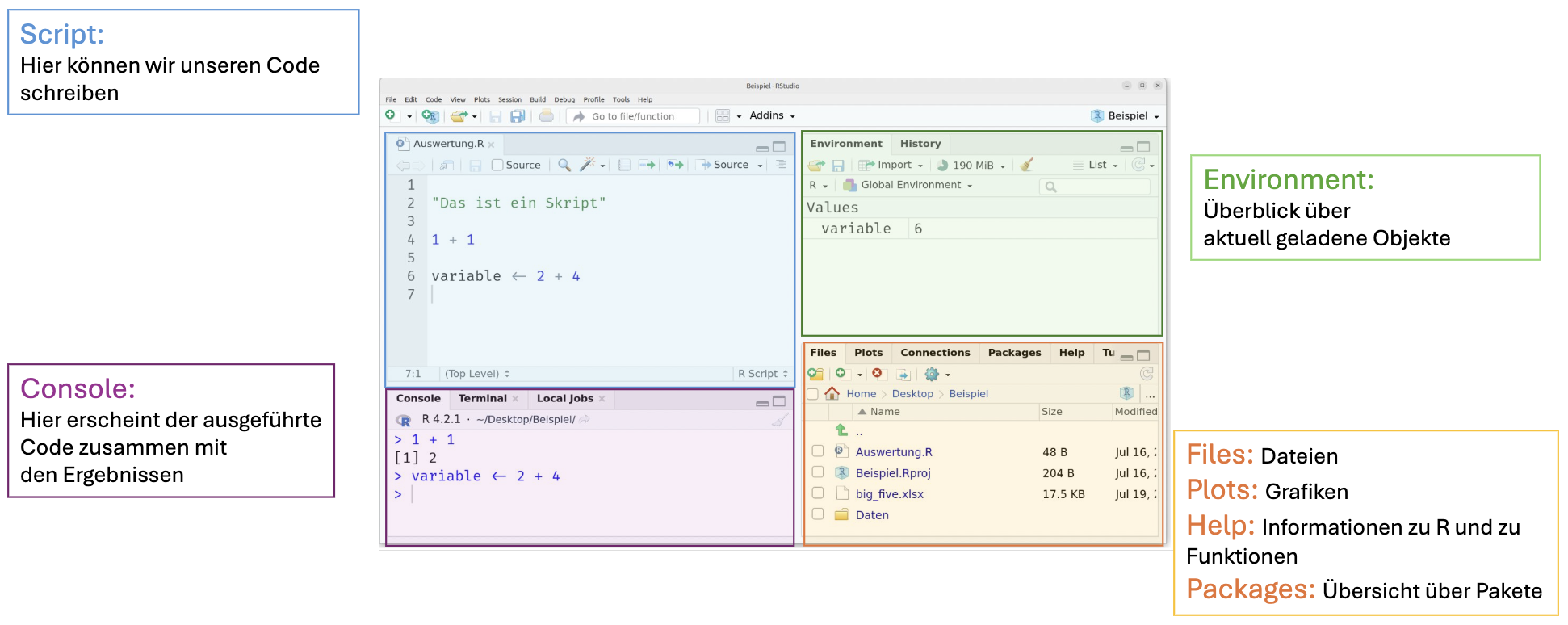
Next we open RStudio by clicking on the RStudio shortcut on the desktop, in the Start menu on Windows or in the Finder under Programs on Mac. When we open RStudio for the first time, the window is divided into the following three areas:
1.2 R as a Calculator
After opening RStudio, we can directly enter and run R commands/code in the window called Console (bottom left). To get started, we use R like a calculator to execute simple calculations. Type…
…in the Console and confirm the input using the Enter- or Return key (↵).
NoteNote
All R commands that we execute in the Console or scripts (we will find out what that is later) ausführen, will be in grey boxes in this tutorial.
1 + 8[1] 9Right below these boxes is the output (the result) of the executed command, which appears in the console in the next line after pressing the ↵ key. Before the result, you will always see a [1] displayed. We can ignore why the reason for this for now.
You can copy the code in the gray boxes by hovering the top right corner of the box and clicking on the copy icon. Then you can insert the code in your console (or script) with the command command + v on Mac or Ctrl + v on Windows.
Copy Code from the Website
Using the symbols on our keyboard we can execute the most important calculation types:
| Symbol on the Keyboard | Calculation/Operation |
|---|---|
+ |
Addition |
- |
Subtraction |
* |
Multiplication |
/ |
Division |
^ |
Exponentiation |
. |
Decimal point |
( and ) |
Structure of the calculation (Parentheses) |
sqrt() |
Square root |
log() |
(Natural) Logarithm |
CautionTry it out!
7 / 8Solution
[1] 0.8751.6 * 7Solution
[1] 11.2log(54)Solution
[1] 3.9889843^2 Solution
[1] 9(3 + 6) * 4Solution
[1] 363 + 7 * 4Solution
[1] 311.3 Logical Comparisons
We can compare two numbers in R and determine whether they are equal or unequal. We can also check whether a number is larger or smaller than another number. Such a question is then answered in R with either Yes (TRUE) or No (FALSE). Such comparisons are called logical comparison and are not limited to numbers (more about this later).
For example, if we’re interested in whether the number 7 is greater than the number 3, we can find out with the code 7 > 3:
7 > 3[1] TRUESince 7 is actually larger than 3, R gives us the response TRUE.
| Symbol on the Keyboard | Calculation or Operation |
|---|---|
== |
Equal |
!= |
Not equal |
> or < |
Greater or less than |
>= or <= |
Greater or equal to, or less than or equal to |
WarningWarning
To check if two numbers are identical, you have to use the operator == and get the return value TRUE (yes, the numbers are identical) or FALSE (no, the numbers are not identical). The individual = assigns a value to a variable (more about that later).
CautionTry it out!
8 > 7Solution
[1] TRUE3 > 4Solution
[1] FALSE3 <= 4Solution
[1] TRUE4 >= 4Solution
[1] TRUE6 == 7Solution
[1] FALSE6 != 7Solution
[1] TRUE8 != 8Solution
[1] FALSE
TipCombined comparisons with logical AND or logical OR
In addition to the simple logical comparisons from above, it is also possible to combine several logical comparisons. As a link, the logical AND as well as the logical OR are particularly relevant.
| Symbol on the Keyboard | Operation | Meaning |
|---|---|---|
& |
logical AND | Are both comparisons true? |
| |
logical OR | Is at least one of the comparisons true? |
In response to a combined logical comparison you get the return value TRUE or FALSE again. To make sure that R evaluates all symbols in the order we want, it can be useful to place brackets.
Example 1:
Is the number 7 greater than 5 AND is the number 9 less than 8?
(7 > 5) & (9 < 8)[1] FALSEExample 2:
Is the number 7 greater than 5 OR is the number 9 smaller than 8 (or both)?
(7 > 5) | (9 < 8)[1] TRUE1.4 Data Types Part 1
In the following we want to introduce you to the most important data types that we will encounter in our work with R.
numeric, integer, double
As we have seen in section 1.2, we can handle the data type “number” in R. For this type of variable, the term numeric is used. In some situations, R differentiates further whether it is an integer number (integer) or a decimal number (double). With each of these three data types, mathematical calculations can be made. For our applications, it usually doesn’t matter whether a number of R is understood as numeric, integer or double. Therefore, we will not discuss the differences in detail.
logical
In section 1.3 we received an information as response to a logical comparison, which can have only two values: TRUE or FALSE. This information has the data type logical in R. If the data type logical is stored for a value, R knows that only these two values are possible.
NoteNote
In fact, some mathematical calculations are also possible with the data type logical. How is that possible? In R, the logical value TRUE is understood as \(1\), the value FALSE as 0. Thus, the calculation TRUE \(+\) TRUE would have to result in \(2\):
TRUE + TRUE[1] 2This property of logical values may seem meaningless at first. However, we can make use of it on many occasions. For example, for any given amount of logical values, we could simply add up all the elements to find out how many elements of this set have the value TRUE.
character (string)
Another important function of R is handling text, which can vary greatly in length—from a single letter to an entire book. Because the order of letters is crucial for readability, text is referred to as strings. In R, the terms character and string are used interchangeably.
Due to the variable length of text, it is necessary to clearly mark where a string begins and ends. This is done using quotation marks "" placed around the text.
"This is my text"[1] "This is my text"Text cannot, of course, be used to make meaningful mathematical calculations, which is why the attempt leads to an error message that part of the calculation is not a number (non-numeric):
"This is my text" + 1Error in "This is my text" + 1: non-numeric argument to binary operator1.5 Assignments
Everything we work with in R is referred to as an object. For example, the result of a logical comparison is an object of type logical. Often, we don’t want to create objects just once and immediately use them; instead, we may want to perform further calculations with them later. For this, we can consciously create objects with names we assign, using what is called an assignment. This allows us to reuse the created and named objects without needing to re-execute the original command.
The assignment is done using the assignment arrow <- (a “lesser than”, directly followed by a “minus”). To the left of the arrow is the object name, which we later use to access the contents of an object. To the right of the arrow is the operation, which provides us as a result the content we want to save. Once we have created the object, it can be found in the Environment window (top right in RStudio). Here you can also find useful information about the object, such as its data type.
An Example
We want to run the operation \(\sqrt{x}\) für \(x = 7\) once and save the result as an object called “A”.
Typically, the programming process is:
- Determine the object name
- Assignment arrow
- Operation
A <- sqrt(7)Assignment
If we want to find out if the assignment has worked and the object A now has the number value of the square root of $7, we can simply run the object A. That is, we enter A after the assignment into the Console and press the Enter key:
A <- sqrt(7)
A
[1] 2.645751If we now only execute the command to the right of the assignment, we see as the result the same number value:
sqrt(7)[1] 2.645751
NoteNote
If we execute the assignment command in the Console, not will be displayed which specific value has been assigned exactly. With the assignment
A <- sqrt(7)we have only instructed R to perform the assignment. We have not given the command to display the specific value. The content of the object is only displayed when we either type in and run the object on the left of the assignment arrow A or the command on the right of the assigment arrow sqrt(7) in the console.
A[1] 2.645751sqrt(7)[1] 2.645751An object can also be overwritten by assigning a new content to it with the assignment arrow. However, the old object is then lost. Therefore, when assigning an object, we have to be aware of whether we’re already using the selected name elsewhere and whether we really want to overwrite the object for good. An overview can be found in the Environment window, because all created objects are listed there.
It is recommended to choose clear and meaningful object names, so you intuitively know the content of the object. E.g., pers_ID <- 123456 for assigning a person ID to an object.
NoteNote
The naming of objects is left to the user’s judgment. Assign the names that best describe the content of the named object for you. However, some characters are not allowed. An object name may usually not contain spaces or hyphens and not start with a digit or an underscore.
Allowed:
my_object <- 4
my.object <- 4
my2ndobject <- 4
objectNumber2 <- 4
Nicht Erlaubt:
my object <- 4
my-object <- 4
2ndObject <- 4
_objectNumber2 <- 4
TipReserved Object Names
In addition to the above rules, there are some specific words that are not allowed as object names because they are reserved for special objects. You can display the list of all reserved words using the following command.
?Reserved
CautionTry it out!
- Calculate \(16^3\) and assign the result to the object \(z\).
- Calculate the square root of \(z\) uand assign the result to the object \(y\).
- Calculate the natural logarithm of \(y\) and assign the result to the object \(x\).
- Perform steps 1 - 3 without assigning intermediate results in one line of code and compare the result with the value stored in \(x\).
Solution
z <- 16 ^ 3
y <- sqrt(z)
x <- log(y)
x
[1] 4.158883log(sqrt(16 ^ 3))[1] 4.158883Of course it is also possible to assign any other data type to an object. For example, if we save text in an object, this object will have the type character. We can find information on the data type contained in an object in the Environment window.
Create a Character Object
2 Reproducible work with RStudio
2.1 R Scripts
So far, we have programmed in the Console. In theory, this would be sufficient to use all functions of R. However, this approach is not recommended! As soon as we close RStudio, all our calculations are lost and are not easily reproducible.
Using R in the Console is like shouting individual tasks to our butler James while decorating the ballroom. James immediately carries out each task as we call it out. A more efficient approach would be to think through everything we want to accomplish, write a list of tasks, and hand it to James. He would then complete each task in the specified order.
The advantage of this approach is that we can revisit the list the next day to see exactly which steps were needed to decorate the ballroom in exactly the same way as before.
Such a procedure is also efficient when using R. The list of work assignments for our Butler R is called Script.
Create a Script
To create a new script, we click on File > New File > R Script.
Alternatively, we click on  and choose R Script. The new script will open in the upper left area.
Create a Script
When we first opened RStudio after the installation, wthe screen was divided into three areas. After creating a script, a fourth area appears at the top left:
TipRStudio Fenster anpassen
The following GIF shows how we can change the size of the individual windows in RStudio.
Change Window Sizes

You can also arrange the Console on the right side of the screen next to the script. This can be useful if we want to see both the script and the console window unfolded large. To arrange the console to the right we go to the menu bar > Tools > Globlal Options > Pane Layout. Here we can select the window arrangement and confirm with Apply.
Arrange Console on the Right
In the script, we can now write all the commands that we would like to execute. Unlike in the Console, however, pressing the `Enter’ key does not execute the command, but it simply results in a line break and we can write another command in the next line.
The script is a collection of commands that are performed to reach a specific goal in a specified order (line by line from top to bottom).
If we want to run a line of the script, we can place the cursor in that line (e.g., by clicking somewhere in the line with the mouse) and then:
- press the key combination Ctrl + Enter (or Ctrl + Return on some keyboards). On a Mac, Command + Enter also works.
- click the
 icon in the top right corner of the script window.
If we want to run multiple lines or specific parts of one or more lines, we can highlight the desired commands and then execute them using either option 1 (Ctrl + Enter) or option 2 (clicking on )
Execute a Script
CautionTry it out!
Open a new script in RStudio
Copy the following lines and paste them into the new script.
x <- 4
y <- 5
x + y # Addition 1
x <- x + y
x + y # Addition 2
Select all lines in the script and run the code with Ctrl-Enter (Mac: command-Enter). What do you notice?
Solution
x <- 4
y <- 5
x + y # Addition 1
[1] 9x <- x + y x + y # Addition 2[1] 14Addition 1 and 2 have different results, because the value of object x is changed between the two calculations.
Swap the third (
x + y) and fourth line (x <- x + y), select the entire code again and execute it. What do you notice?Solution
x <- 4
y <- 5
x <- x + y
x + y # Addition 1
[1] 14x + y # Addition 2[1] 14Addition 1 and 2 now have the same results because the value
xwas changed before the first addition. Although the same commands were executed in sum, the order of the commands makes a crucial difference.
Save Script
To save a script, we have several options:
- In the menu bar: File > Save
- Using the key combination Strg + s (Windows and Mac) or command + s (Mac only)
- In R Studio below the symbol
 in the upper left corner.
2.2 Dealing with the Workspace
When we work in R, we usually create different objects (e.g. x <- 42), which are then displayed in our Environment window in RStudio. At some point we are finished with our statistical analysis for today and want to close RStudio. If we close RStudio, we are asked by the program if we want to save the Workspace, which contains all our R objects from the Environment window (and a few other things).
Unlike our R script, we do not want to save the Workspace (in 99% of cases)!
NoteWhy don’t we save the workspace?
- Only what is written in our R script is reproducible! If we have tried things in the R Console, deleted or adapted commands in our script, we don’t know exactly how the objects came about in the Environment.
- Therefore, it is good practice to force ourselves to include all essential steps for the analysis in the script by starting with a “fresh” working environment (= empty Environment) every time we work with R.
If we saved the Workspace when closing RStudio, all R objects from the previous session would automatically reload upon reopening. While this might seem convenient, it often causes issues in practice.
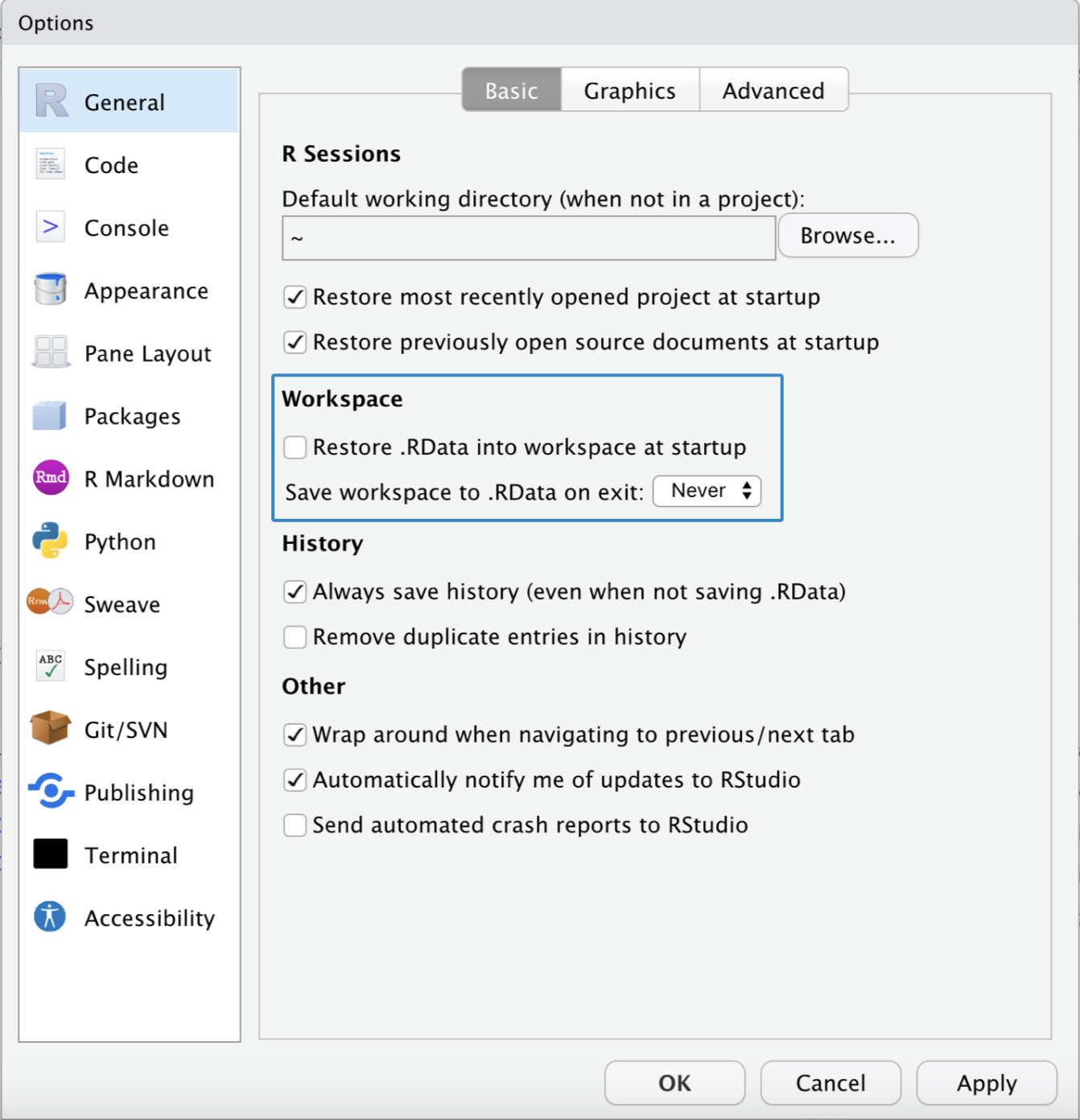
Adjusting Workspace Settings
In RStudio’s settings, we can specify that…
- no workspace should be loaded when opening, and
- when closing RStudio the workspace is not saved and we are no longer asked about it.
To do this we click on Tools > Global Options and select the settings marked blue in the picture below.
CautionTry it out!
Adjust the workspace settings in RStudio as described.
Create at least one R object, e.g. with the command
x <- 10. Close RStudio and note that you are no longer asked if you want to save the workspace (if you have made changes to an R script, you will still be asked if you want to save the script).Reopen RStudio and confirm that the previously created R object no longer exists. You can either try to display the object (e.g. by entering the name of the object in the Console and pressing Enter) or you can make sure that the Environment window in RStudio is empty.
2.3 Restarting R in the background
Even while working in RStudio, it makes sense to reset R , and create a “fresh working environment” (= empty Environment) regularly. We want to make sure that the code in our R script works as expected and that we can actually reproduce all essential analysis steps.
Instead of closing and reopening RStudio, we can instead restart R in the background by either…
- clicking on Session > Restart R or
- pressing the key combination command + Shift + 0 für Mac oder Strg + Shift + F10 für Windows verwenden.
After that, we can either…
- manually re-run our code in the script step by step, or
- use the key combination command + Shift + Enter (Mac) or Strg + Shift + Enter (Windows) to execute the complete currently opened script.
CautionTry it out!
Create a new R script containing only the following three lines:
x <- 1
y <- 2
x + y
Run the three commands in a row in the script line by line.
Enter the following command directly in the Console:
y <- xRe-run the third line of the script and compare the result with the result that one would expect only knowing what’s in the script.
Restart R in the background by using the described key combination.
Re-execute the complete script by using the described key combination. Check the result.
3 Working with Data
3.1 Functions
Arguments
Functions perform operations for us by giving them certain input values, so-called Arguments. This is comparable to the mathematical functions that specify which calculations are to be made with the Argument \(x\) to get a result \(y\), e.g.
Functions perform operations for us by accepting specific input values, known as arguments. This is similar to mathematical functions, which specify the calculations to be performed with the argument \(x\) to produce a result \(y\), e.g.,:
\[ f(x) = x^2 + 5 \] Similarly, functions in R can process one or more arguments and return results such as mean values, sums or more complex operations.
An Example
One relatively simple function is the exponential function \(e^x\). Its only argument is the exponent.
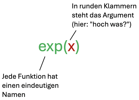
Using the exponential function in R for \(x = 1\):
exp(1)[1] 2.718282It is often useful to use a result of functions as an argument for another function. These functions are then nested in a certain order.
An Example
To calculate \(e^{\sqrt{x}}\) we would first calculate the square root of \(x\) with the function sqrt(x) and then insert the result as an argument in the exponential function exp():
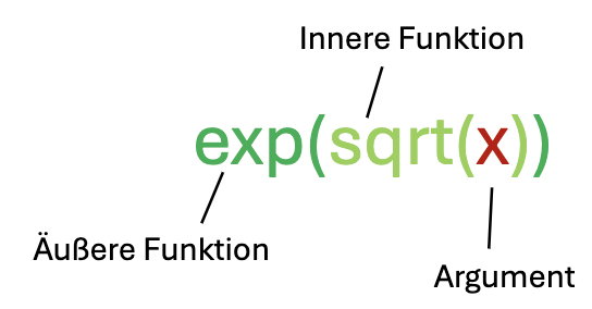
WarningWarning
The order of nesting plays a role, e.g.,:
\(e^{\sqrt{1}} \neq \sqrt{e^{1}}\)
exp(sqrt(1))[1] 2.718282sqrt(exp(1))[1] 1.648721In mathematics, it is also possible to process more than one argument in one function, such as in the equation for a plane in three-dimensional space:
\[ f(x, y) = 2x + 3y \] Similarly, in R, many functions require multiple arguments. These arguments are separated by commas within a command and have distinct names to differentiate them. Some arguments have default settings, which R uses if no value is specified for that argument.
An Example
This becomes clearer using the example of the round(x, digits) function, which rounds a number to any number of decimal places. As the first argument, we pass the number to be rounded to the function, as the second argument, the number of decimal places. The name of the argument that determines the number of decimal places is digits. The default (the default if you don’t pass an argument for digits) is zero. So the number will be rounded to zero decimal places if the digits argument is not specified.
.png)
The round(4.12345, digits = 2) function rounds the number 4.12345 to two decimal places, i.e. to 4.12.
NoteDo arguments have to be named?
You will notice as we proceed that arguments can be specified in two ways. In the example above, round(4.12345, digits = 2), the first argument, the number to be rounded (4.12345), is provided unnamed, while the second argument, the number of desired decimal places (2), is provided named with digits =.
In principle, both approaches are possible for any argument, but they will only produce the same result if the expected order of arguments for the command is followed. If arguments are left unnamed, the command cannot distinguish whether 2 refers to the number to be rounded or the number of decimal places. We can clarify this for the command by adhering to the order of arguments specified in the corresponding help page (see section 3.1.2).
The process becomes less error-prone and significantly clearer if we follow the following convention:
- The first argument of a command (the main argument with which the command works) is not named.
- All further arguments that we want to specify are named with the corresponding name (e.g.
digits =).
CautionTry it out!
round(4.12345, 2)[1] 4.12yields the same result as
round(x = 4.12345, digits = 2)[1] 4.12On the other hand,
round(2, 4.12345)[1] 2does not lead to the desired result.
The command assumes that the number 2 should be rounded to 4.12345 decimal places. While specifying decimal places for an integer makes no sense, the command resolves this by simply ignoring the decimal places and attempting to round 2 to four decimal places instead.
By naming the arguments, we could do without the correct order:
round(digits = 2, x = 4.12345)[1] 4.12Although this reversal of the order would technically work, it is rather uncommon. A widely accepted style convention suggests that the main argument of the command, which is expected in the first position, should remain unnamed, while all subsequent arguments can be provided in any order but should be explicitly named:
round(4.12345, digits = 2)[1] 4.12
TipFunctions without Arguments
In R there are also functions without any argument, such as:
Sys.time() # the point in time at which this command was executed[1] "2025-11-13 16:25:05 CET"On a technical level, whenever something happens in R (calculating, displaying, or processing any kind of information), a function is executed.
Help
If we want to understand how a function works, such as the names of its arguments, we need to consult the help documentation. The help section can be found in the “multifunction window” at the bottom right, under the Help tab.
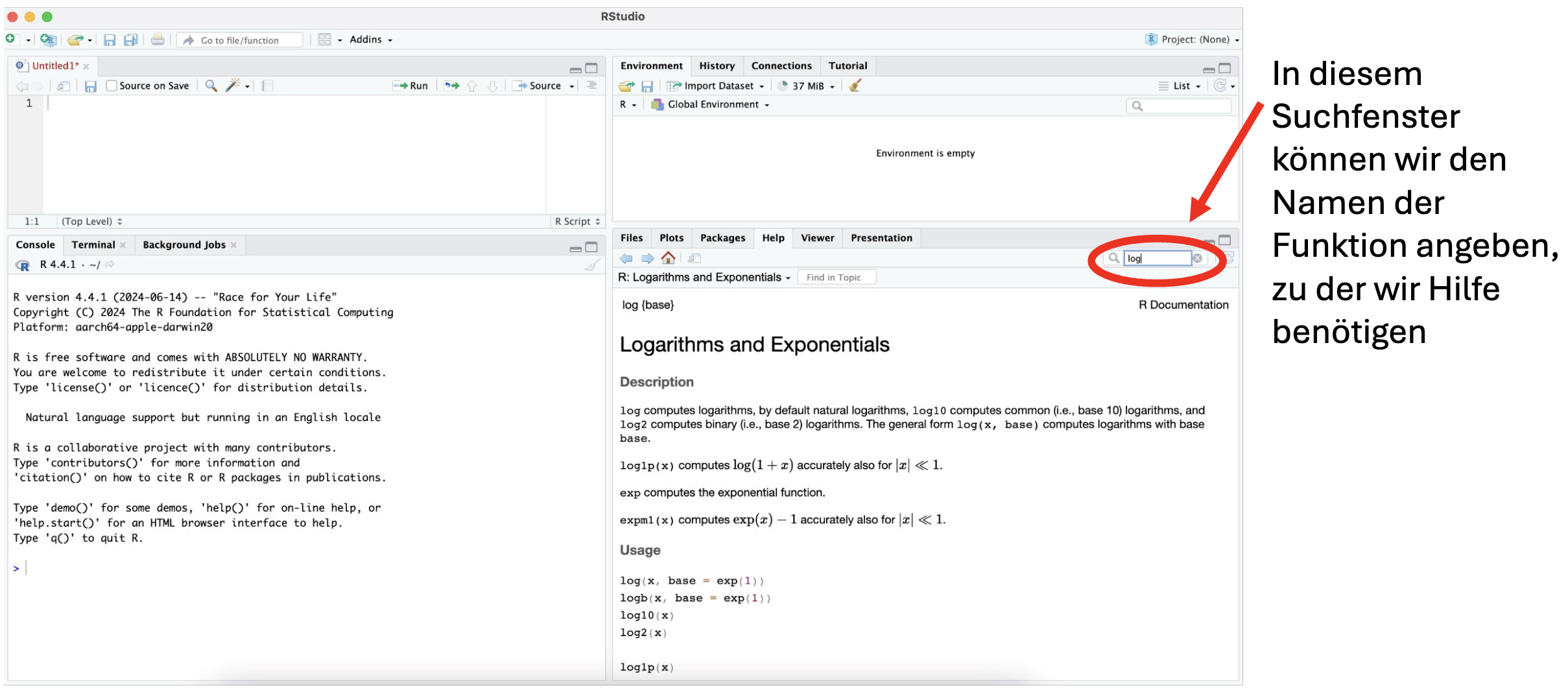
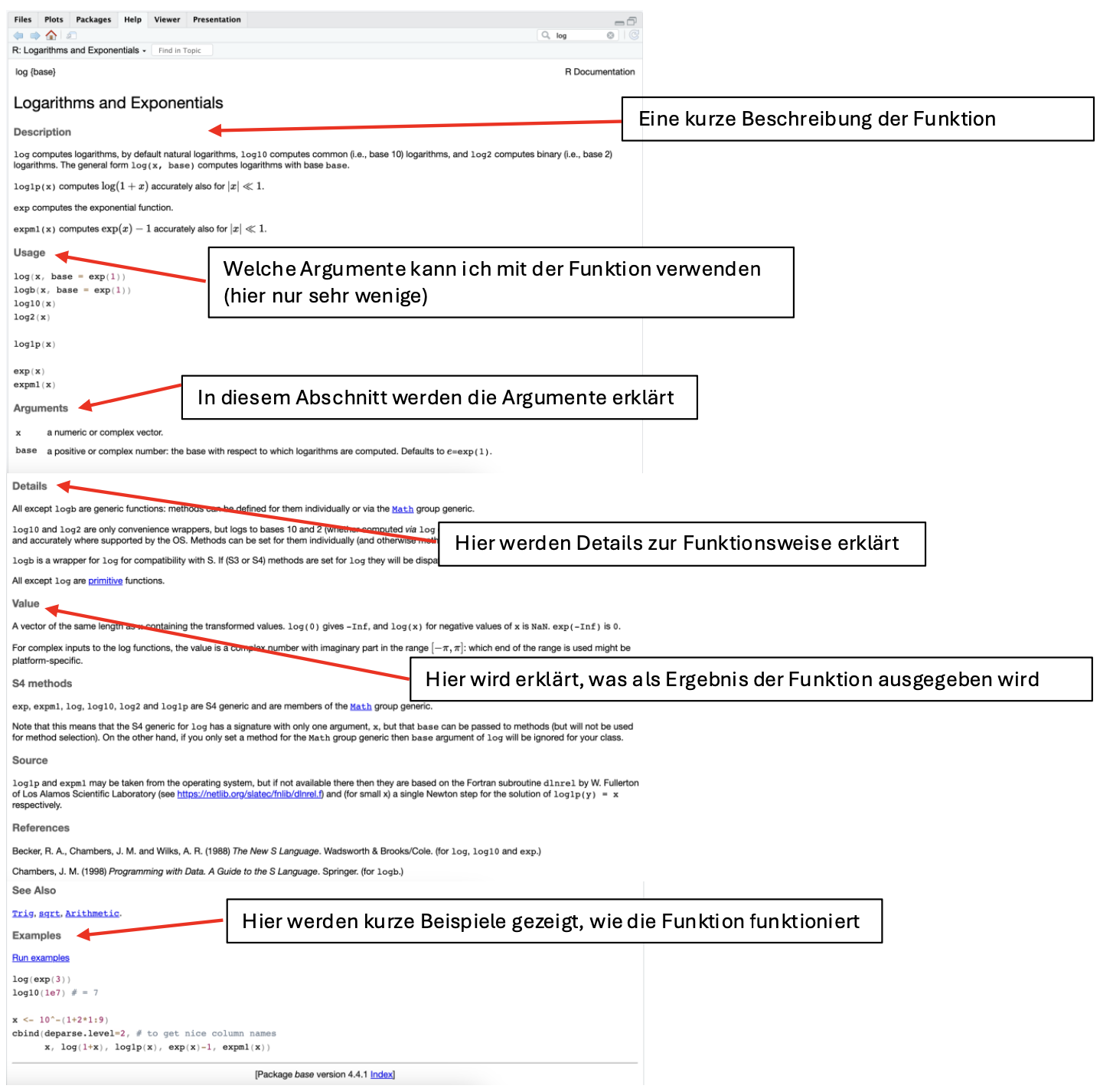
We can open the help window even faster by typing in a question mark right before the function’s name in the Console (e.g., ?log) and executing the command.
On the help page, we can see under Description or Usage that the log() function, by default, calculates the natural logarithm (which is almost always the one needed in statistics). However, we could specify a different base using the base argument.
CautionTry it out!
Find out why why the following calculation prints 0as result using the help function.
round(0.5, digits = 0)[1] 0Solution
On the help page for ?round, under Details, it says:
Note that for rounding off a 5, the IEC 60559 standard (see also ‘IEEE 754’) is expected to be used, ‘go to the even digit’. Therefore round(0.5) is 0 and round(-1.5) is -2.
The help in R is only useful if we already know the name of a function. But what do we do if we don’t know the name of a function (or have forgotten it)? In other words, how can we find out in practice which commands or functions in R can help us with a specific task?
Typically, we enter a question formulated as precisely as possible into the search engine of our choice.
WarningUsing AI Tools Instead of Search Engines
Nowadays, instead of using a search engine, we can enter our R-related questions into an AI tool like ChatGPT. In fact, ChatGPT is quite knowledgeable about the basics of R. However, we should still be cautious and verify whether the suggested commands actually do what we want. For example, it is relatively common for ChatGPT to invent functions for more complex problems that don’t actually exist in R.
Oftentimes, such a search reveals that a useful function for us is included in a specific R package.
Packages
When we install R, a large number of functions are already available in the base version. However, it is possible to significantly extend the functionality through so-called packages. Most of these packages are continuously maintained and expanded by a large group of developers and are freely available to all R users.
Often, packages are created by researchers for a specific purpose and contain a series of commands designed to build upon each other and help solve a typical problem.
If we want to use commands from a package, we first need to download (“install”) the package. This can be done either with the command install.packages("PACKAGENAME") or by using the Packages tab in the bottom-right panel of RStudio.
Installing Packages
In both cases, we need to know the exact name of the package. For example, if we enter the name incorrectly in the command install.packages("PACKAGENAME") (or forget the quotation marks), the command will fail:
install.packages("Psych") # the package is called "psych" with a lowercase pWarning: package 'Psych' is not available for this version of R
A version of this package for your version of R might be available elsewhere,
see the ideas at
https://cran.r-project.org/doc/manuals/r-patched/R-admin.html#Installing-packagesWarning: Perhaps you meant 'psych' ?
WarningCaution
The error message…
Warning: package 'Psych' is not available for this version of R
…does not mean that our version of R is outdated!
In this case, we simply made a typo (R is correct: there is no package called ‘Psych’ for our version of R, but there is one called ‘psych’).
Just as we only need to install programs on our computer once, packages also generally need to be installed only once to be used repeatedly. However, after an update to R (not RStudio), it is often necessary to reinstall previously installed packages.
To use the commands from a package, we first need to make it available to R. This process is called loading the package. The best way to do this is with the command…
library(PACKAGENAME)… which we normally write in the very beginning of our script, so we don’t forget to load the necessary packages.
Of course, the command must not only be in the script, it also has to be executed!
NoteNote
A package usually only has to be installed once, but after each restart of R or RStudio it needs to be loaded again so that we can use the commands in it.
An Example
For our example, we want to use the so-called logistic function:
\[ f(x) = \frac{1}{1 + e^{-x}} \]
Since we read online that the package psych includes a command logistic() that can compute this function, we will install and load this package. Before the package is installed and loaded, we cannot use the command it provides.
logistic(0)Error in logistic(0): could not find function "logistic"Therefore, we install the package once, as described above, via the Packages tab or using the following code:
# install once:
install.packages("psych")
If installing the package worked, we can now load the package:
# load:
library(psych)
and use the command logistic()
logistic(0)[1] 0.5
CautionTry it out!
If you haven’t already completed the steps described above, try using the function
logistic()before installing and loading thepsychpackage.
Then, install the package as described above.
Load the package as described above.
Execute the following commands:
logistic(0)
logit(0.5) # this is the inverse function
Close RStudio and try running the commands from step 4 again.
Solution
Without loading the package, it won’t work:
logistic(0)Error in logistic(0): could not find function "logistic"logit(0.5) # this is the inverse functionError in logit(0.5): could not find function "logit"Only if we load the package in the script beforehand, it works:
library(psych)
logistic(0)
[1] 0.5logit(0.5) # this is the inverse function[1] 0
WarningCaution
When installing a package using the function install.packages("PACKAGENAME"), the package name must be in quotation marks. However, when loading it with the function library(PACKAGENAME), quotation marks are not required.
NoteNote
When we open a script that attempts to load a package that has not yet been installed, RStudio notifies us. At the top of the script, a message appears: “Package PACKAGENAME required but is not installed. Install Don’t Show Again”. Here, we can simply click on Install to install the package directly.
TipWriting Custom Functions
If we need a function that has not yet been implemented in R and is not included in any package, it is also possible to write our own functions.
This allows us to execute specific code repeatedly without having to rewrite (or copy) the entire code each time.
Functions are also objects and can be stored in variables. We then call the function using these variables. A function is structured as follows:
function_name <- function(<function parameters>) {
    # Code
}
To call a function, you add () after the function name.
Now, we can write a simple function that executes the logistic function described above when called:
logistic_function <- function(number) {
    1 / (1 + exp(-number))
}
This code does not produce any output yet because, although we have written the function, we have not called it. To execute the function, we use its name and add () with the argument the function should work with (just like with the functions we’ve used so far).
When writing the function, we specified in the () after function that it should work with an object called number. In the next line, within the {}, we performed the operation (\(\frac{1}{1 + e^{-x}}\)) using this object number, which defines the operation our function is intended to perform.
A brief test of the function shows that it does what it’s supposed to do:
logistic_function(number = 0)[1] 0.5Most functions work with multiple arguments. For example, we can write a function that returns the sum of two numbers (essentially recreating the existing sum() function). We use the two placeholders x and y as arguments, which will later be replaced by the numbers we want to add when we call the function:
my_sum <- function(x, y) {
    x + y
}

my_sum (x = 3, y = 5)
[1] 8
CautionTry it out!
Write a function square() that takes a number as an argument and returns its square.
Solution
square <- function(x) {
  x * x
}

square(x = 3)
Write a function logit_function() that calculates the inverse of the logistic function: \[ f(y) = ln(\frac{y}{1 - y}) \]
Solution
logit_function <- function(number) {
  log(number / (1 - number))
}

logit_function(number = 0.5)
3.2 Data Structures
Simple Data Structures: Vectors
So far, we have only stored a single value when assigning an object. However, we often want to work with a whole set of values. To store a series of values of the same data type, we use vectors. You’ve probably encountered the term “vector” in math class.
A point in three-dimensional space can, for example, be precisely specified with one vector containing three pieces of information (the \(x\)-, \(y\)-, and \(z\)-coordinates).
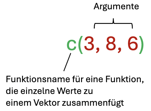
If we want to combine multiple components (e.g., numbers) into a vector in R, we use the function c().
As we learned earlier with function arguments, the individual values are separated by commas within the function.
As we know from math class, we can also perform calculations with vectors. For example, we can subtract two vectors of the same length from each other
\[ \vec{v} = \begin{pmatrix} 3 \\ 8 \\ 5 \end{pmatrix} - \begin{pmatrix} 1 \\ 5 \\ 2 \end{pmatrix} = \begin{pmatrix} 3 - 1 \\ 8 - 5\\ 5 - 2 \end{pmatrix} = \begin{pmatrix} 2 \\ 3 \\ 3 \end{pmatrix} \] or subtract a specific number from each element of a vector
\[ \vec{v} = \begin{pmatrix} 3 \\ 8 \\ 5 \end{pmatrix} - 2 = \begin{pmatrix} 3 - 2 \\ 8 - 2\\ 5 - 2 \end{pmatrix} = \begin{pmatrix} 1 \\ 6 \\ 3 \end{pmatrix} \]
In R, we first need to create the desired vector using c() and can then perform calculations with it as usual:
c(3, 8, 5) - 2[1] 1 6 3As we can see, vectors in R are always displayed as rows, but this makes no difference for our purposes.
For longer vectors, it can be useful to first store the vector in an object and then perform the operation using that object.
# Abspeichern eines Vektors in einem Objekt
mein_Vektor <- c(3, 8, 5)
mein_Vektor - 2
[1] 1 6 3Both approaches lead to the same result, so it’s up to us which one we choose.
In math class, you have probably only encountered vectors with numbers, which can be used for calculations. However, the structure of a vector is useful for many purposes. A vector, in general terms, is an object that contains any number of elements of the same type in a fixed order. As we will see, it is also very useful to group multiple elements into a vector for other data types (such as logical values or characters) in many situations.
A vector always has exactly one data type. For example, a vector of type logical can be created in much the same way as with numbers, using the c() command:
c(TRUE, FALSE, TRUE)[1] TRUE FALSE TRUEThe “identifier” for logical values is that all TRUE and FALSE values are spelled correctly (i.e., all uppercase with no typos).
Creating a vector of type character works in exactly the same way. Here, the “identifier” for character values is the use of "" around each element:
c("Homer", "Marge", "Bart", "Lisa", "Maggie")[1] "Homer" "Marge" "Bart" "Lisa" "Maggie"
WarningCaution
Different data types cannot be mixed in a vector.
If we include different data types in a vector, R tries to find a common denominator, which usually results in the type character.
c(3, "word", TRUE) [1] "3" "word" "TRUE"When we run this code and display the “mixed” vector, we see that all elements are enclosed in "". This indicates that the number 3 and the logical value TRUE have now been converted to character values, losing their original properties.
The conversion of data types often happens without R issuing a warning, making it easy for us as users to overlook. However, converting data to character can result in the loss of certain properties. For example, we can no longer perform mathematical operations, such as addition, on the character value "3".
CautionTry it out!
Assign the birth year of three (fictional) people to the vector birth_year.
How old did all three people turn in 2023?
Assign the names of the people from (1) to the vector names in the same order.
Solution
birth_year <- c(1998, 2002, 1988)

2023 - birth_year
[1] 25 21 35names <- c("Markus", "Philipp", "Moritz") names[1] "Markus" "Philipp" "Moritz"
More Complex Data Structures: Data Frames and Lists
data.frame
So far, we’ve seen that we can group data into one-dimensional objects, such as vectors. However, we can also create multidimensional structures, such as an object consisting of multiple vectors. One particularly important structure is called a data frame (or data.frame), which is similar to a matrix (R also has matrices, but since we rarely use them, we won’t cover them here).
A data frame consists of rows and columns. The columns are all the same length but can contain data of different types. For example, one column Names can contain character values, and another column Age can contain numeric values. This makes a data frame the most useful and important type of data structure for us. For instance, we can store information for multiple individuals (each row corresponding to one individual) across various attributes (name, age, grade, level of psychological symptoms, etc.) in columns of different types. The data frame ensures that the information for each individual is always correctly aligned. For example, the third value in the first column (e.g., name) corresponds to the same person as the third value in the third column (e.g., grade), and so on.
We can create a data frame ourselves using the data.frame() function. This function takes an argument for each desired column in the dataset. Naming the arguments (e.g., Age =) ensures that each column gets a meaningful header:
df <- data.frame(
  Name = c("Tom", "Paula", "Mia", "Jonas"),
  Age = c(21, 22, 21, 20) # Important: stick to the order of the names!
  )

df # executing the object displays the data frame
Name Age
1 Tom 21
2 Paula 22
3 Mia 21
4 Jonas 20We can add new variables to our data frame using the $ symbol. The following code adds a new column containing the favorite food of our individuals.
When doing this, we must ensure that the new vector has as many entries as there are rows in the data frame (in this case, 4). The first entry of the vector corresponds to the first individual, the second entry to the second individual, and so on.
df$Favorite_Food <- c("Pizza", "Döner", "Ice Cream", "Pizza")

df
Name Age Favorite_Food
1 Tom 21 Pizza
2 Paula 22 Döner
3 Mia 21 Ice Cream
4 Jonas 20 Pizza
NoteData are normally not typed into R directly!
In this example, we manually entered the data into df to demonstrate what a data frame is with a simple example. In practice, nobody enters a real dataset directly into R! Instead, datasets are typically either generated automatically (e.g., by software for online surveys) or entered manually into a spreadsheet program (e.g., Excel or LibreOffice). These prepared datasets (sometimes called “raw data”) are then “imported” into R for statistical analysis or further processing. We will learn how to import datasets later in Part 2 of the tutorial.
list
A list is a flexible data structure that can contain objects of different types (e.g., numbers, characters) or even different structures (e.g., vectors, data frames). Just like with a data frame, simple names for the list elements can be assigned directly within the list() function.
my_list <- list(number = 1256, name = "Tomas", vector = c(1, 2, 5, 6))

my_list
$number
[1] 1256
$name
[1] "Tomas"
$vector
[1] 1 2 5 6An important difference from data frames is that list elements can have different lengths. The results of more complex analyses are often stored in lists, and we may want to access their individual elements.
Indexing: Accessing Elements of an Object
Indexing Vectors
So far, we have seen how to combine data when creating vectors. However, we can also access individual elements of a vector (indexing), for example, if we are only interested in the entry at the second position.
In R, this is done using vector indexing. Square brackets [] are used to access the position we are interested in. Inside the brackets, we specify place of the element we want to select within the vector (e.g., 1 for the first element, 2 for the second element, and so on).
# create example vector
my_vector <- c(3, 8, 5, 7)

# Access the second number
my_vector[2]
[1] 8
TipHow are long vectors displayed in R output?
If we display a long vector in R, the output no longer fits in a single line.
long_vector <- 100:200 # `100:200` generates all integers from 100 to 200.
long_vector
[1] 100 101 102 103 104 105 106 107 108 109 110 111 112 113 114 115 116 117
[19] 118 119 120 121 122 123 124 125 126 127 128 129 130 131 132 133 134 135
[37] 136 137 138 139 140 141 142 143 144 145 146 147 148 149 150 151 152 153
[55] 154 155 156 157 158 159 160 161 162 163 164 165 166 167 168 169 170 171
[73] 172 173 174 175 176 177 178 179 180 181 182 183 184 185 186 187 188 189
[91] 190 191 192 193 194 195 196 197 198 199 200Now that we’ve learned about the [] syntax, we can understand for the first time what the numbers in square brackets (e.g., [1], [19], etc.) in the output mean. These numbers indicate the position of the first element displayed at the beginning of each line in the output. This is very helpful for navigating long outputs more quickly.
In our example, long_vector, the 1st element is the number 100 ([1] 100), the 19th element is the number 118 ([19] 118), and so on. We can verify this using the indexing we just learned:
long_vector[19][1] 118A single number is treated by R as a vector with just one element.
This is why [1] is always displayed when a single number is output, even though it’s not particularly helpful…
To access multiple entries of a vector, we create a vector within the square brackets [] and specify the positions of the entries we want to select as the elements of that vector.
my_vector <- c(3, 8, 5, 7)

# accessing the second and fourth number
my_vector[c(2, 4)]
[1] 8 7
WarningCaution!
If we want to access multiple elements of a vector, we must not forget to use the vector created with c() inside the square brackets [c(x, y)]. It is not possible to access multiple elements directly within the square brackets without the intermediate step of creating a vector with c() (e.g., [2,3,4]). We will see why later.
With square brackets, we can not only view individual values but also modify them. The following code assigns the value 4 to the second position of our vector, overwriting the value 8.
my_vector <- c(3, 8, 5, 7)

my_vector[2] <- 4

my_vector
[1] 3 4 5 7Indexing Data Frames
We’ve already seen how to use square brackets [] to access individual values in vectors. Similarly, we can use them to access specific values in data frames. This allows us to select a single row, a single column, or an individual value (a combination of row and column). Of course, we can also select multiple rows, columns, or values.
The square brackets take two arguments because data frames have two dimensions. As with other commands, the arguments are separated by a comma.
The first argument specifies the row, and the second argument specifies the column:
df[row, column]Remember: We already created the following data frame in section 3.2.2.1:
df Name Age Favorite_Food
1 Tom 21 Pizza
2 Paula 22 Döner
3 Mia 21 Ice Cream
4 Jonas 20 PizzaHere, for example, we can select all columns for the first person (i.e., the first row) by passing row 1 as the first argument inside square brackets and leaving the second argument after the comma blank. Leaving it blank means that all columns are selected:
df[1, ] Name Age Favorite_Food
1 Tom 21 PizzaOr, if we are only interested in the age of all individuals, we select the second column. Here, we leave the first argument blank (as we want to select all rows) and pass column 2 as the second argument:
df[ , 2][1] 21 22 21 20If we are specifically interested in the age of the first individual in our data frame, we can select this single value by passing row 1 as the first argument and column 2 as the second argument:
df[1, 2][1] 21Similar to vectors, we can also select multiple rows or columns here by combining them into a vector:
df[c(1, 2), c(1, 2)] Name Age
1 Tom 21
2 Paula 22Before and after the comma [ , ], only one piece of information is allowed. Therefore, we need to group all the information regarding the rows and columns into a single object (in this case, a vector).
If we know the names of the columns but not their positions, we can also access them directly by their names:
df[ , c("Age", "Favorite_Food")] Age Favorite_Food
1 21 Pizza
2 22 Döner
3 21 Ice Cream
4 20 Pizza
NoteNote
If we recall, we saw that it is not possible to access the first three entries of a vector using my_vector[1, 2, 3].
Now that we’ve looked at indexing data frames, we understand that the arguments within square brackets refer to the dimensions.
Indexing Data Frames and Lists using $
In addition to indexing with square brackets [ , ], we can also use column names to extract entire columns. For this, we use the dollar sign $.
df$Name[1] "Tom" "Paula" "Mia" "Jonas"As soon as we type the $ sign, RStudio’s autocomplete suggests all column names from the dataset for selection.
Autocomplete
$-indexing also works with lists. For instance, we can access from the list we created above…
my_list$number
[1] 1256
$name
[1] "Tomas"
$vector
[1] 1 2 5 6… its element called vector like this:
my_list$vector[1] 1 2 5 6Conditional Indexing of Data Frames
So far, we have mainly looked at how to select specific columns. Now, we will see how to select individuals from our data frame who meet certain conditions.
In the following example, we want to select all individuals from our data frame whose favorite food is pizza. In a large dataset, it would be very time-consuming to manually determine the positions of these individuals and write them into a vector.
Instead, we can identify the positions of individuals whose favorite food is pizza using a logical comparison:
df$Favorite_Food == "Pizza"[1] TRUE FALSE FALSE TRUEHere, we check for each row whether the column FavoriteFood in the data frame df contains the entry “Pizza.” As described in section 1.3, the return value of a logical comparison is either TRUE or FALSE. This gives us information for each row of the data frame about whether the person listed in that row specified “Pizza” as their favorite food. We want to select rows where the result is TRUE and exclude those where it is FALSE.
The information about where TRUE appears can now be directly used in our indexing. To do this, we insert the code performing the logical comparison directly into the code responsible for selecting specific rows. This is placed before the comma within the selection df[ , ]:
df[df$Favorite_Food == "Pizza", ] Name Age Favorite_Food
1 Tom 21 Pizza
4 Jonas 20 Pizza
CautionTry it out!
What code retrieves the data from the FavoriteFood column only for 21-year-olds?
Solution
df[df$Age == 21, "Favorite_Food"][1] "Pizza" "Ice Cream"
TipIndexing with logical AND or logical OR
Conditional indexing becomes even more useful when we consider that we can combine multiple logical comparisons using logical AND (symbol & in R) or logical OR (symbol | in R).
Remember that this is our example data frame:
df Name Age Favorite_Food
1 Tom 21 Pizza
2 Paula 22 Döner
3 Mia 21 Ice Cream
4 Jonas 20 PizzaExample 1:
Display the names of all individuals that are older than 20 AND younger than 22.
df[df$Age > 20 & df$Age < 22, "Name"][1] "Tom" "Mia"Example 2:
Display the names of all individuals whose favorite food is pizza OR that are 21 years old.
df[df$Favorite_Food == "Pizza" | df$Age == 21, "Name"][1] "Tom" "Mia" "Jonas"3.3 Practical Functions for Data Frames
We have already learned what functions and arguments are. This included mathematical functions like exp(), as well as the round() function and the c() function for creating vectors.
In our practical work, we will almost always work with data stored in R as a data.frame. Since data frames are so common, we will explore some useful functions for working with them. Later, our datasets will often be large, with hundreds of rows and columns, making it impossible to manually determine what is contained in a data frame or whether there are any irregularities. For this reason, there are several functions that we can use directly with a data frame as an argument to obtain general information about it.
str()describes the structure of an object, such as its data type and the number of elements it contains. This function is extremely useful when working with all types of objects (not just data frames).
nrow()returns the number of rows in a data frame, andncol()returns the number of columns.
head()displays the first six rows of a data frame (useful only if there are more than six rows), whiletail()shows the last six rows.
summary()summarizes the information contained in an object (not limited to data frames).
For data frames, this function tries to describe each column in a meaningful way.
WarningDon’t Force Yourself to Memorize Commands and Functions!
At first, it might seem like “learning R” means memorizing lots of commands and function names.
However, that’s not how programming works in practice. The most important thing is to understand how R works (e.g., what data frames are and how the [ , ] syntax functions). Even experienced R users don’t know the names of all available functions, and it’s perfectly normal to look up information repeatedly while programming (see, for example, section 3.1.2 on how to do this efficiently). Commands and functions that you use frequently will naturally become familiar over time.
In the following examples, we apply the functions listed above to the previously created data frame df to display general information about its structure:
str(df)'data.frame': 4 obs. of 3 variables:
$ Name : chr "Tom" "Paula" "Mia" "Jonas"
$ Age : num 21 22 21 20
$ Favorite_Food: chr "Pizza" "Döner" "Ice Cream" "Pizza"In the output of str(), we see that our data frame has 4 rows (obs. stands for observations) and 3 columns (variables). The first column is called Name and contains character values (chr). The second column is called Age and contains numeric values (num for numeric). The third column is called Favorite_Food and again contains character values.
nrow(df)[1] 4ncol(df)[1] 3If we have a larger dataset than our example and only want to view the first or last six rows, we can use head() or tail(). However, since df in our example only has four rows, this is meaningless in this case.
head(df) Name Age Favorite_Food
1 Tom 21 Pizza
2 Paula 22 Döner
3 Mia 21 Ice Cream
4 Jonas 20 Pizzatail(df) Name Age Favorite_Food
1 Tom 21 Pizza
2 Paula 22 Döner
3 Mia 21 Ice Cream
4 Jonas 20 PizzaWe can get a summary for each column in the dataset using the summary() command. This command can also be applied to objects other than data frames and will frequently be used in statistical analyses.
summary(df) Name Age Favorite_Food
Length:4 Min. :20.00 Length:4
Class :character 1st Qu.:20.75 Class :character
Mode :character Median :21.00 Mode :character
Mean :21.00
3rd Qu.:21.25
Max. :22.00 Depending on the data type of a column, the summary looks different. For numeric columns like Age, we get a series of descriptive statistics, such as the mean (Mean). For text columns like Name and Favorite_Food, the summary is not particularly useful, as summary() does not handle character values well. It would be more meaningful if these two columns were stored as factor instead.
3.4 Data Types Part 2
Factors
In section 1.4, we introduced the three data types numeric, logical, and character. The logical type with TRUE and FALSE values is particularly useful when data can only take on two values (e.g., “Is a person’s age > 18?” or “Does a person have a specific condition or not?”). When more than two values are possible, we need another solution: the factor data type.
A factor can have a predefined set of values (levels) that represent the possible data categories. It is also possible for a level to be defined but not actually occur in our dataset.
An Example
Let’s say we conducted a survey where participants were asked which psychology program they are enrolled in. We know that LMU offers only a limited selection of psychology programs (e.g., “Bachelor Major,” “Bachelor Minor,” “Master”), even though not all of these categories may appear in our survey data.
For example, among our three respondents, two are enrolled in the Bachelor Major program, and one is in the Master program:
study_program <- factor(c("Bachelor Major", "Bachelor Major", "Master"), # Caution: don't forget the c()!
                      levels = c("Bachelor Major", "Bachelor Minor", "Master"))

study_program
[1] Bachelor Major Bachelor Major Master
Levels: Bachelor Major Bachelor Minor MasterThe created object study_program is now of the factor type thanks to the factor() command. As the first argument of this command, we provided the responses from our three individuals as a vector of type character. As the second argument, levels =, we specified the theoretical categories that could exist.
What’s the benefit of specifying levels that are not observed in the data? By including “Bachelor Minor” as a level, even though it does not appear in the data, R “knows” that this is a possible category that wasn’t observed. When using a command like creating a frequency table, R will now indicate that the first category “Bachelor Major” was observed twice, the third category “Master” was observed once, and the second category “Bachelor Minor” was not observed at all:
table(study_program) # displays a simple frequency tablestudy_program
Bachelor Major Bachelor Minor Master
2 0 1 When performing statistical analyses with data stored as text, we sometimes need to decide whether the character data type is sufficient or if we need to store the text data as a factor.
TipSome R Functions Require Factor Instead of Character
Later, certain functions in R will require that columns in our data frames containing text information are stored as factors instead of characters.
We’ll demonstrate this with a small example:
The commonly used function summary() can display helpful summaries for many different types of objects. However, as we saw earlier, when we apply this function to our previously created data frame df, the summary of the two character columns, Name and Favorite_Food, is not particularly useful for us…
summary(df) Name Age Favorite_Food
Length:4 Min. :20.00 Length:4
Class :character 1st Qu.:20.75 Class :character
Mode :character Median :21.00 Mode :character
Mean :21.00
3rd Qu.:21.25
Max. :22.00 The summary becomes more meaningful when we convert the two columns to a factor using the factor() command:
df$Name <- factor(df$Name)
df$Favorite_Food <- factor(df$Favorite_Food)
summary(df)
Name Age Favorite_Food
Jonas:1 Min. :20.00 Döner :1
Mia :1 1st Qu.:20.75 Ice Cream:1
Paula:1 Median :21.00 Pizza :2
Tom :1 Mean :21.00
3rd Qu.:21.25
Max. :22.00 As we can see, the summary()command displays a useful frequency table for factor columns.
Missing Values
So far, we have always assumed that all individuals we survey provide complete responses. For instance, in the example above, all three respondents told us which study program they are enrolled in. In section 3.2.2.1, all four individuals in our example provided their name, age, and favorite food. However, this is often not realistic, as in many cases respondents give incomplete answers.
An Example
Let’s assume that when creating our data frame df, Tom, Paula, and Mia provided their ages, but Jonas did not want to share his age. We can’t simply leave out Jonas’s age, as this would reduce the number of values to three, which would then be incorrectly aligned with the wrong individuals in the rows. Therefore, we need a way to indicate during the creation of the data frame that a value should be present but is unknown.
This can be done using a so-called missing value, represented in R by the combination of letters NA. We can now insert an NA in place of Jonas’s value in the Age column:
df <- data.frame(
  Name = c("Tom", "Paula", "Mia", "Jonas"),
  Age = c(21, 20, 21, NA) # Important: stick to the order of the names!
  )

df # executing the object displays the data frame
Name Age
1 Tom 21
2 Paula 20
3 Mia 21
4 Jonas NA
WarningCaution
If NAs are present in the data, commands might not work as we expect. However, many commands have specific arguments that tell them how to handle NAs.
An Example
The sum() function allows us to add multiple values. If we pass the Age column df$Age to this function, it will try to sum all the values in this column:
sum(df$Age)[1] NAThe result is also an NA?! This happens because the function doesn’t know how to compute the sum of three numbers and one unknown value.
If we want the function to ignore the NA and sum the three remaining values instead, we can achieve this by using the argument na.rm = TRUE:
sum(df$Age, na.rm = TRUE)[1] 62You can find out the name of the argument that defines how a command handles missing values in the help page for the respective function (e.g., ?sum, see section 3.1.2).
4 Common Mistakes
Below, we’ve compiled a list of the most common mistakes we all make when working with R (and that’s perfectly normal!). Keep these in mind when something doesn’t work as expected in R.
Typos
df[ , c("Favoriet_Food")]Error in `[.data.frame`(df, , c("Favoriet_Food")): undefined columns selectedMisspelled Column Name
If we misspell a column name while selecting the column, R won’t find the column.
Name <- c("Tom", "Pia", "Nelly")
Age <- c(21, 24, 33)

Data <- data.frame(name, Age)
Error in eval(expr, envir, enclos): object 'name' not foundMisspelled Column Name while Selecting
Forgotten Comma
Data <- data.frame(Name Age)Error: <text>:1:25: unexpected symbol 1: Data <- data.frame(Name Age ^An unexpected symbol often means that a comma between arguments within a function was forgotten.
Forgotten Comma
Forgetting quotation marks for strings
#| error: true
Name <- Tom
instead of
Name <- "Tom"`
Forgetting Quotation Marks for Strings
Forgetting the closing quotation mark
#| eval: false
Name <- "Tom
> Name <- "Tom +This error can be especially confusing because R won’t execute the command until the quotation mark is closed (R assumes the command is incomplete and “waits”). The Console will display
+instead of>and won’t respond to new commands as usual. In this case, the easiest solution is to click into the Console with the mouse and press the Esc key. Afterward, you can re-enter the command correctly.Forgetting the Closing Quotation Mark
Forgetting a closing parenthesis
#| eval: false
Name <- c("Tom", "Pia"
> Name <- c("Tom", "Pia" +Similar to the previous error, the Console will display
+until the parenthesis is closed. In this case, it’s again easiest to click into the Console with the mouse and press the Esc key.Forgetting a Closing Parenthesis
Misspelled function name
Data <- dataframe(Name, Age)Error in dataframe(Name, Age): could not find function "dataframe"Misspelled Function Name

Two things could have happened here:
- The function is misspelled (as in this case).
- The function is spelled correctly, but the package containing the function has not yet been loaded using
library(PACKAGENAME).
- The function is misspelled (as in this case).
Comments
In many cases, it makes sense to include comments in our script so that other people or we can later understand what was calculated.
Comments are written after a
#character. When executing the code, R knows that this is a comment and does not execute the line.For comments that go over more than one line, there must be a
#at the beginning of each line. It is also possible to write a comment directly behind an executable command:We can see that only the code before the
#is executed.When you’re just learning R, it makes sense to comment on what the commands in your script do. The more familiar you get with R, the less you will need such comments, because the information what your code does is in the commands themselves. (After all, you could always find out how the commands work by researching them later). Therefore, it is more useful to comment on why a certain code is necessary to achieve the goal of your analysis (and why you didn’t choose another way). Such information is not immediately apparent from the code itself and it is quite amazing how quickly you forget what you were thinking about when you were programming something.