# You need to have the ggplot2 package installed
install.packages("ggplot2")R Tutorial (Part 2): Efficient Workflows for Dataset Handling
1 Workflow So Far
In Part 1 of our R tutorial, we not only covered the basics of how R works but also familiarized ourselves with some workflows for the efficient use of R and RStudio in chapter 2 Reproducible Work with RStudio.
If you don’t clearly remember the following topics, we strongly recommend reviewing them:
We have learned…
- what an R script is and why it’s better not to enter all commands directly into the Console.
- what the Workspace is, and we configured RStudio so that it does not automatically save it when the program is closed.
- how to restart R regularly in the background and why this is essential to ensure that your R script is truly reproducible.
Here in Part 2, we will build on this foundation to learn what an RStudio project is and how it can help us import and analyze empirical datasets in R.
TipFor Interested Readers: Additional Resources on R
For more detailed information on the topics covered here and many others, we recommend the freely available online book R for Data Science (2e) by Hadley Wickham, Mine Çetinkaya-Rundel, and Garrett Grolemund.
If you already have extensive experience with other programming languages or enjoy exploring the inner workings of R in the greatest possible detail, we suggest the freely available online book Advanced R by Hadley Wickham.
2 Workflow with Projects
2.1 What Is an RStudio Project?
In practice, working with R almost always involves importing a dataset into R and performing various analyses on the data.
Such datasets are typically stored as files on your hard drive, for example, a file named Pounds.csv.
To import the dataset, you need to tell R where this file is located.
This can be quite cumbersome in practice and makes the analysis error-prone, especially if, for instance, you want to share your R script with a colleague who naturally has a different folder structure on their computer.
To address this, it’s good practice to use so-called projects from the start. These projects greatly simplify working with multiple files (which is almost always relevant in real-world analyses).
An RStudio project is essentially just a new folder on your hard drive that contains all the files (R scripts, datasets, figures, etc.) related to a specific analysis project (e.g., your thesis). In addition, the RStudio project folder includes a shortcut that allows you to open the project directly in RStudio.
NoteWhen Should I Create a New Project?
Defining what constitutes a “project” and when it’s worth creating a new RStudio project for an analysis can be difficult to generalize. One large RStudio project containing all the statistical analyses for your entire degree program would almost certainly be “too big,” while a project dedicated to just one exercise sheet from a statistics seminar would likely be “too small.” In practice, beginners often create RStudio projects that are “too large,” trying to include too many unrelated analyses in one project. For example, a project focused on the final report for a statistics seminar would be a reasonable size, while combining all exercises, notes, and unrelated analyses from the entire seminar into one project would likely be too much.
2.2 Creating a New RStudio Project
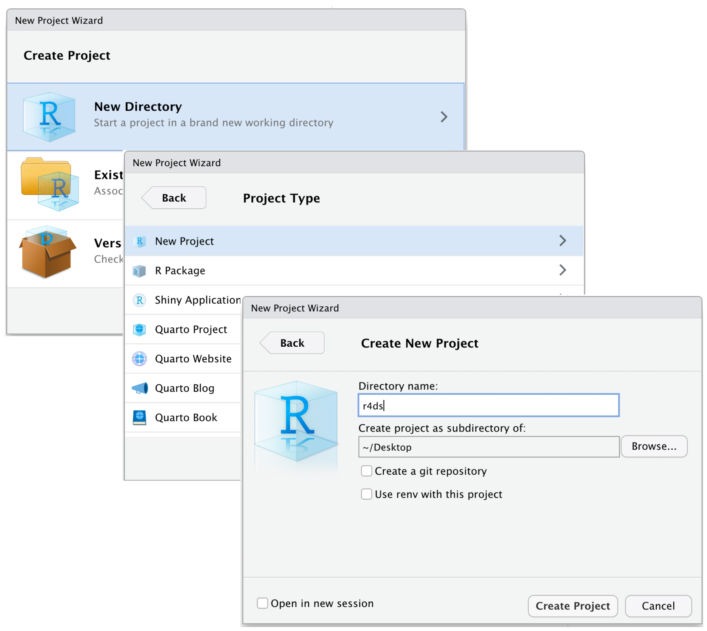
To create a new project in RStudio:
- Click on File > New Project,
- Enter a name for your project folder,
- Choose where to save the project folder on your computer, and
- Click Create Project.
This process is illustrated in Figure 1.
After creating the new project, we can see the project folder in RStudio’s Files pane. Initially, the folder contains only a shortcut, a file with the .Rproj extension, named the same as the project folder.
After closing RStudio, we can reopen the project by double-clicking the .Rproj file on our computer.
When a project is open in RStudio and we save a file, such as an R script or a plot, these files are saved in the project folder by default. This makes it easy to keep all files related to the project organized in one place.
CautionTry it out!
Create a new RStudio project named
R_Intro(or another name you prefer). Think carefully about where to save the project on your computer so that you can easily locate the folder the next time you want to open it.Close RStudio.
Download the file
msleep.Rand move it to the newly created project folder. (Note: If the file opens in your browser instead of downloading, go back to the link, right-click, and select Save link as).Open the project by double-clicking the
R_Intro.Rprojfile.Verify that you can see the downloaded file in the Files pane in RStudio.
In the Files pane, click on the R script
msleep.R.Run the commands in the
msleep.Rscript. It doesn’t matter if you don’t fully understand what all the commands do. If an error occurs, it’s likely because a required R package is missing. Use the information in the R script to identify the missing package, install it, and then rerun the commands in the script.Solution
Take a look at the Files pane in RStudio and observe what has changed in your project folder.
Solution
The script has created and saved two new files: the dataset
msleep.csvand the plotmsleep.png. The project folder was automatically chosen as the storage location.
Solution as GIF
3 Workflow for Importing Datasets
3.1 Importing a Dataset in .csv Format
Datasets are often stored in files with formats like .csv, .xlsx, or .sav.
R provides functions to import files in each of these formats (and many others).
Here, we will start by focusing on .csv files.
In the English standard, the CSV format uses commas (,) to separate entries from different cells in a table, while decimal points in numbers are written with a period (.). However, programs set to German often handle things a bit differently: cells are separated by a semicolon (;), and decimals are marked with a comma (,).
Both types of CSV files can be imported into R without any issues. However, the difference in delimiters must be accounted for. Use the read.csv() function for the English format and read.csv2() for the German format. If the wrong function is used, the data will not be read into R in a meaningful way.
To import a dataset, we need to specify the file path in the R command, including the file name and its exact location on the computer.
However, if 1) we are working within an RStudio project, and 2) the file is located directly in the project folder, it’s sufficient to provide only the file name (including the file extension) when importing.
For instance, we can download the dataset Pounds.csv, move it to the project folder, and import it into R using the read.csv2() function.
We can then assign the imported data to an object pounds using <-, allowing us to continue working with the data in R.
Then, we can for example use the head() function to view the first six rows of the dataset:
pounds <- read.csv2("Pounds.csv")
head(pounds)
group treat motivat pounds
1 1 0 4 15
2 1 0 4 17
3 1 0 4 15
4 1 0 4 17
5 1 0 4 16
6 1 0 6 18If we’re unsure about the CSV format of the data, we can simply try both functions (read.csv() and read.csv2()) and see which one imports the data in the correct format.
WarningThe Numbers App on Mac Breaks .csv Files!
On many Macs, the Numbers app is the default program for opening .csv files outside of RStudio, such as when double-clicking a CSV file in the Finder. For reasons no one quite understands, the Numbers app modifies any opened CSV file in a way that makes it unreadable by R. This alteration happens the moment you open the file, even if you don’t save it afterward.
To avoid this frustrating issue, you must ensure that you do not open CSV files with Numbers. If this does happen by mistake during our seminar, we recommend simply re-downloading the file. If Numbers is set as the default program for opening CSV files on your Mac, we suggest changing the default program. Instructions on how to change default programs on a Mac can be found here.
3.2 The Working Directory
…or: “Why is it enough to specify just the file name when importing files in an RStudio project?”
When working in R, there is always a folder on your computer where R looks for files (e.g., to import them) or saves files (e.g., when saving a plot created in R). This folder is called the Working Directory.
In an RStudio project, the project folder is automatically set as the Working Directory. When importing a file, we only need to specify the file path relative to the Working Directory. This means:
- If the file is located directly in the project folder, it is sufficient to specify only the file name (including the file extension) when importing, e.g.,
pounds <- read.csv2("Pounds.csv").
- If the file is in a subfolder within the project folder (e.g., a folder named
data), you need to include the subfolder in the file path, e.g.,pounds <- read.csv2("data/Pounds.csv").
This highlights the major advantage of RStudio projects:
If all files are stored within the project folder, our analyses will work regardless of where the project folder is located on our computer. This means we can move the project folder anywhere on our computer or even send it as an email to colleagues without breaking the file paths.
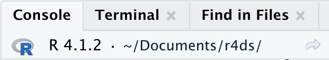
NoteChecking the Working Directory
You can check the current location of the Working Directory either by looking at the top of the Console window, as shown in Figure 2, or by running the R command getwd().
CautionTry it out!
Download the file
HSB.csvand move it to the project folder.Import the file
HSB.csvusing the functionread.csv2()and assign the data to the objecthsb.Create a summary of all variables in the HSB dataset using the command
summary(hsb).Solution
hsb <- read.csv2("HSB.csv")
summary(hsb)
School Minority Sex SES Min. :1224 Length:7185 Length:7185 Min. :-3.760000 1st Qu.:3020 Class :character Class :character 1st Qu.:-0.540000 Median :5192 Mode :character Mode :character Median : 0.000000 Mean :5278 Mean :-0.001857 3rd Qu.:7342 3rd Qu.: 0.600000 Max. :9586 Max. : 2.690000 MathAch Size Sector PRACAD Min. :-2.83 Min. : 100 Length:7185 Min. :0.0000 1st Qu.: 7.28 1st Qu.: 565 Class :character 1st Qu.:0.3200 Median :13.13 Median :1016 Mode :character Median :0.5300 Mean :12.75 Mean :1057 Mean :0.5345 3rd Qu.:18.32 3rd Qu.:1436 3rd Qu.:0.7000 Max. :24.99 Max. :2713 Max. :1.0000 DISCLIM MeanSES Min. :-2.4200 Min. :-1.190000 1st Qu.:-0.8200 1st Qu.:-0.320000 Median :-0.2300 Median : 0.040000 Mean :-0.1319 Mean : 0.006224 3rd Qu.: 0.4600 3rd Qu.: 0.330000 Max. : 2.7600 Max. : 0.830000In exercise 7 from section 2.2, the file
msleep.csvwas created in your project folder. If you don’t have this file, you can instead download it here. Import the filemsleep.csvand assign the data to the objectmsleep_data. Try both read.csv functions to determine which one is suitable for importing the dataset.Solution
msleep_data <- read.csv("msleep.csv")
head(msleep_data)
name genus vore order conservation 1 Cheetah Acinonyx carni Carnivora lc 2 Owl monkey Aotus omni Primates <NA> 3 Mountain beaver Aplodontia herbi Rodentia nt 4 Greater short-tailed shrew Blarina omni Soricomorpha lc 5 Cow Bos herbi Artiodactyla domesticated 6 Three-toed sloth Bradypus herbi Pilosa <NA> sleep_total sleep_rem sleep_cycle awake brainwt bodywt 1 12.1 NA NA 11.9 NA 50.000 2 17.0 1.8 NA 7.0 0.01550 0.480 3 14.4 2.4 NA 9.6 NA 1.350 4 14.9 2.3 0.1333333 9.1 0.00029 0.019 5 4.0 0.7 0.6666667 20.0 0.42300 600.000 6 14.4 2.2 0.7666667 9.6 NA 3.850Calculate the mean of the column
sleep_total.Solution
mean(msleep_data$sleep_total)[1] 10.43373Bonus: Calculate the mean of the column
sleep_totalonly for the rows in the dataset where the columnordercontains the value"Primates".Solution
mean(msleep_data[msleep_data$order == "Primates", "sleep_total"])[1] 10.5Bonus - Open End: The online storage service Zenodo is widely used by researchers to make their data publicly available. If you want to practice importing datasets with even more examples, you can find many recent psychological datasets in .csv format here.